Particle loading
Particles in EPOCH belong to particle species which can be controlled by the species block. In these examples, we show how to load macro-particles in various configurations. These macro-particle objects behave as single particles in the code, but represent many real particles for the current solver. The examples on this page set up simulations in epoch2d, but they may be modified for use in the 1d or 3d codes.
Uniform load
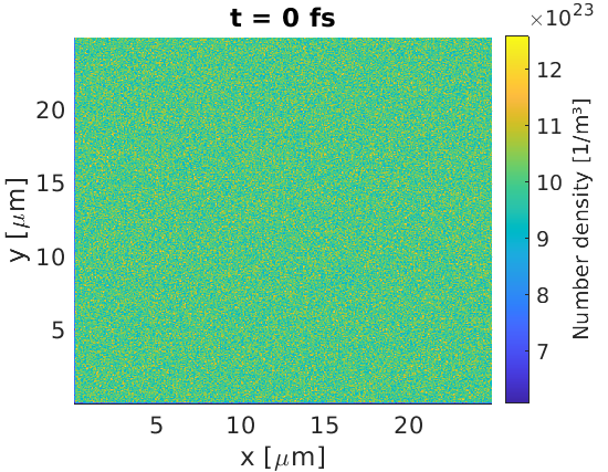
This basic input deck sets up a uniform density of electrons over the full simulation window. We create 10 macro-particles per cell, for a density of $10^{24}\text{ m}^{-3}$. The cell sizes are $dx = dy = 50\text{ nm}$ and $dz = 1 \text{ m}$, since cell sizes in omitted dimensions default to 1 metre. Hence, we expect $2.5\times 10^9$ real electrons per cell, so each macro-electron should represent around $2.5\times 10^8$ real electrons.
begin:control
    nx = 500
    ny = 500
    t_end = 1.0e-15
    x_min = 0
    x_max = 25e-6
    y_min = 0
    y_max = 25e-6
    stdout_frequency = 100
end:control

begin:boundaries
    bc_x_min = open
    bc_x_max = open
    bc_y_min = open
    bc_y_max = open
end:boundaries

begin:species
    name = Electron
    mass = 1.0
    charge = -1.0
    npart = 50 * nx * ny
    density = 1.0e24
    temp_ev = 1000
end:species

begin:output
    dt_snapshot = t_end
    number_density = always
end:output
Basic target
The shape of the target can be controlled by using maths parser expressions in the density key. For example, a $5 \text{ }\mu\text{m}$ target slab can be defined according to
begin:control
    nx = 500
    ny = 500
    t_end = 1.0e-15
    x_min = 0
    x_max = 25e-6
    y_min = 0
    y_max = 25e-6
    stdout_frequency = 100
    npart = 50 * (5.0e-6/(x_max-x_min)) * nx * ny
end:control

begin:boundaries
    bc_x_min = open
    bc_x_max = open
    bc_y_min = open
    bc_y_max = open
end:boundaries

begin:species
    name = Electron
    mass = 1.0
    charge = -1.0
    frac = 0.8
    density = if (x gt 15.0e-6, 1.0e24, 0)
    density = if (x gt 20.0e-6, 0, density(Electron))
    temp_ev = 1000
end:species

begin:species
    name = Carbon
    mass = 22033.0
    charge = 6.0
    frac = 0.2
    density = density(Electron) / 6
    temp_ev = 1000
end:species

begin:output
    dt_snapshot = t_end
    number_density = always
end:output
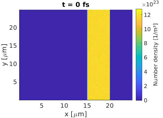
This target contains both electrons, and fully ionised carbon ions. The number
of macro-particles loaded has been set to ensure there are 50 particles per
cell, accounting for the fact most cells are in vacuum. The if command in
EPOCH uses an if-else format, such that the line:
density = if (x gt 20.0e-6, 0, density(Electron))
means that for cells with $x>20\text{ }\mu\text{m}$, set the density to 0, and in all other cells, set the density to what it was already (no change).
Rotated target
Let us take the basic target, and rotate it about the point $(15.0,12.5)\text{ }\mu\text{m}$. To do this, we can set new functions in a constant block to help.
We may use a rotation transformation
$x' = x\cos(\theta) + y\sin(\theta)$
$y' = -x\sin(\theta) + y\cos(\theta)$
to obtain $x$ and $y$ co-ordinates in a rotated co-ordinate system, which makes the writing of the input.deck more straightforward. An example input.deck is provided:
begin:constant
    x0 = 15.0e-6
    y0 = 12.5e-6
    theta = 30.0 / 180.0 * pi
    x_rot =  (x-x0)*cos(theta) + (y-y0)*sin(theta)
    y_rot = -(x-x0)*sin(theta) + (y-y0)*cos(theta)
end:constant

begin:control
    nx = 500
    ny = 500
    t_end = 1.0e-15
    x_min = 0
    x_max = 25e-6
    y_min = 0
    y_max = 25e-6
    stdout_frequency = 100
    npart = 50 * (5.0e-6/(x_max-x_min)) * nx * ny / sin(theta)
end:control

begin:boundaries
    bc_x_min = open
    bc_x_max = open
    bc_y_min = open
    bc_y_max = open
end:boundaries

begin:species
    name = Electron
    mass = 1.0
    charge = -1.0
    frac = 0.8
    density = if (x_rot gt 0.0, 1.0e24, 0)
    density = if (x_rot gt 5.0e-6, 0, density(Electron))
    temp_ev = 1000
end:species

begin:species
    name = Carbon
    mass = 22033.0
    charge = 6.0
    frac = 0.2
    density = density(Electron) / 6
    temp_ev = 1000
end:species

begin:output
    dt_snapshot = t_end
    number_density = always
end:output
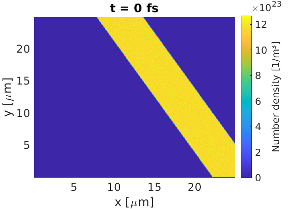
By creating the x_rot, y_rot variables, we can define objects in a rotated
co-ordinate system. In this new system, the x0, y0 point is the origin, and
theta is the rotation amount in radians. The number of loaded macro-particles
has been increased by 1 / sin(theta) to account for the fact that more cells
contain particles than in the non-rotated case.
Periodic structure
We may use a certain trick in the
maths parser to generate
repeating structures. If we wished to add strucutre to the front surface of a
target, where the repeated unit had a size of $y_r$, then a variable y_f
y_f = (y / y_r) - floor(y / y_r)
would continuously repeat from 0 to 1 in each periodic window. This can be used to create a repeating strucutre.
For example, if the user wished to add a stack of half-spheres to the front of the target, they may use:
begin:constant
    x_front = 15.0e-6
    circle_radius = 2.0e-6
    y_r = 2.0 * circle_radius
    y_f = 2.0*((y / y_r) - floor(y / y_r))-1.0
end:constant

begin:control
    nx = 500
    ny = 500
    t_end = 1.0e-15
    x_min = 0
    x_max = 25e-6
    y_min = 0
    y_max = 25e-6
    stdout_frequency = 100
    npart = 50 * (5.0e-6/(x_max-x_min)) * nx * ny
end:control

begin:boundaries
    bc_x_min = open
    bc_x_max = open
    bc_y_min = open
    bc_y_max = open
end:boundaries

begin:species
    name = Electron
    mass = 1.0
    charge = -1.0
    frac = 0.8
    density = if ((x-x_front)^2 + (y_f * circle_radius)^2 lt circle_radius^2,\
                  1.0e24, 0)
    density = if (x gt x_front and x lt (x_front + 5.0e-6), \
                  1.0e24, density(Electron))
    temp_ev = 1000
end:species

begin:species
    name = Carbon
    mass = 22033.0
    charge = 6.0
    frac = 0.2
    density = density(Electron) / 6
    temp_ev = 1000
end:species

begin:output
    dt_snapshot = t_end
    number_density = always
end:output

Note: due to the target complexity, I have not tried to force 50 macro-particles per cell in this simulation.
Load density from file
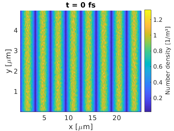
Sometimes a density distribution can be too complicated to set up using the EPOCH maths parser. In this case, EPOCH can read a binary file where the density in each cell is specified.
Binary files can be written by many coding languages. In this example, I used MATLAB to write a sinusoidal density profile to file, using the code provided here. Note the order of numbers being written - we perform a full line of $x$ values first, before moving onto the second line at the next $y$.
nx = 500;
ny = 100;
fileID = fopen('density.bin','w');
for iy = 1:ny
    for ix = 1:nx
        density = abs(sin(ix/20));
        fwrite(fileID,density,'double');
    end
end
fclose(fileID);
An input deck was created to read this binary, where I have specified the full path to the binary file position
begin:control
    nx = 500
    ny = 100
    t_end = 1.0e-15
    x_min = 0
    x_max = 25e-6
    y_min = 0
    y_max = 5e-6
    stdout_frequency = 100
end:control

begin:boundaries
    bc_x_min = open
    bc_x_max = open
    bc_y_min = open
    bc_y_max = open
end:boundaries

begin:species
    name = Electron
    mass = 1.0
    charge = -1.0
    npart = 5 * nx * ny
    density = '/home/examples/density.bin'
    temp_ev = 1000
end:species

begin:output
    dt_snapshot = t_end
    number_density = always
end:output
This yielded the desired output for the density profile
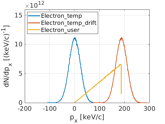
Momentum distributions
While the density key in EPOCH can be used to set up macro-particle positions,
the temperature and drift keys provide momentum distributions. The
temperature key samples a momentum from a relativistic Maxwell-Jüttner
distribution, and drift applies a Lorentz boost to these momenta.
The user may also specify their own momentum distribution, using dist_fn.
A functional form for the momentum distribution can be written in the
input deck, and
EPOCH can sample momenta from this distribution. As an example, say we wanted a
linearly-increasing distribution for the momentum x-component, from $p_x=0$ to
$p_x = p_{max}$
dist_fn = px / p_max
where the maximum value of dist_fn has been set to 1. When sampling, EPOCH
will generate $p_x$, $p_y$ and $p_z$ values within a user-chosen range, and
substitute these into the dist_fn expression yielding a number between 0 and
1. This number corresponds to the probability of keeping the sampled momenta,
or choosing a new set, which is sampled using a uniformly-distributed random
number.
As an example, the following input deck initialises 3 species. One using only temperature, one with the same temperature and drift, and the last using a user-defined function.
begin:control
    nx = 500
    ny = 500
    t_end = 1.0e-15
    x_min = 0
    x_max = 25e-6
    y_min = 0
    y_max = 25e-6
    stdout_frequency = 100
end:control

begin:boundaries
    bc_x_min = open
    bc_x_max = open
    bc_y_min = open
    bc_y_max = open
end:boundaries

begin:species
    name = Electron_temp
    mass = 1.0
    charge = -1.0
    npart = 5 * nx * ny
    density = 1.0e24
    temp_ev = 1000
end:species

begin:species
    name = Electron_temp_drift
    mass = 1.0
    charge = -1.0
    npart = 5 * nx * ny
    density = 1.0e24
    temp_ev = 1000
    drift_x = 1.0e-22
end:species

begin:species
    name = Electron_user
    mass = 1.0
    charge = -1.0
    npart = 5 * nx * ny
    density = 1.0e24
    dist_fn = px / 1.0e-22
    dist_fn_px_range = (0, 1.0e-22)
end:species

begin:output
    dt_snapshot = t_end
    px = always
    weight = always
end:output
Load particles from file
If the user requires spatial and momentum distributions too complicated for the previous methods, then they may perform the ultimate brute-force technique. Using the particles_from_file block the user is able to manually specify the position, momentum and weight of each macro-particle at the start of the simulation.
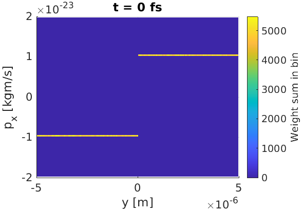
As an example, let us set up a simple simulation where particles above $y=0$ have momentum $p_x = 10^{-23}\text{ kgm/s}$, and where $p_x = -10^{-23}\text{ kgm/s}$ below $y=0$. We will also force a uniform density of macro-particles over the simulation window, and assign each macro-particle a weight of 10. The particle files to achieve this were written by the following MATLAB code
% Simulation parameters
part_count = 1.0e5;
x_min = 0;
x_max = 25.0e-6;
y_min = -5.0e-6;
y_max = 5.0e-6;
px0 = 1.0e-23;

% Set particle properties
x_vals = (x_max - x_min) * rand(1,part_count) + x_min;
y_vals = (y_max - y_min) * rand(1,part_count) + y_min;
w_vals = 10 * ones(1,part_count);
px_vals = px0 * ones(1,part_count);
px_vals(y_vals<0) = -px0;

% Write files
x_file = fopen('x.bin','w');
y_file = fopen('y.bin','w');
w_file = fopen('w.bin','w');
px_file = fopen('px.bin','w');
for i = 1:part_count
    fwrite(x_file,x_vals(i),'double');
    fwrite(y_file,y_vals(i),'double');
    fwrite(w_file,w_vals(i),'double');
    fwrite(px_file,px_vals(i),'double');
end
fclose(x_file);
fclose(y_file);
fclose(w_file);
fclose(px_file);
To load these macro-particles into the simulation, the following input.deck was used
begin:control
    nx = 500
    ny = 200
    t_end = 1.0e-15
    x_min = 0
    x_max = 25e-6
    y_min = -5e-6
    y_max = 5e-6
    stdout_frequency = 100
end:control

begin:boundaries
    bc_x_min = open
    bc_x_max = open
    bc_y_min = open
    bc_y_max = open
end:boundaries

begin:species
    name = Electron
    mass = 1.0
    charge = -1.0
end:species

begin:particles_from_file
    species = Electron
    x_data = "/home/examples/x.bin"
    y_data = "/home/examples/y.bin"
    w_data = "/home/examples/w.bin"
    px_data = "/home/examples/px.bin"
end:particles_from_file

begin:output
    dt_snapshot = t_end
    distribution_functions = always
end:output

begin:dist_fn
    name = y_px
    ndims = 2
    dumpmask = always
    direction1 = dir_y
    direction2 = dir_px
    resolution2 = 100
    range2 = (-2.0e-23, 2.0e-23)
    include_species:Electron
end:dist_fn
Here, we have provided the full paths to the particle file locations. To visualise the distribution of macro-particles in position and momentum space, we output a distribution function to obtain the expected figure.
Self-heating
Low resolution PIC codes can result in self-heating, where macro-particles can gain energy non-physically. To measure its effect, we can simulate a small portion of the simulation and assign periodic boundary conditions. Self-heating can be reduced by using:
- Smaller cell sizes
- More marcro-particles per cell
- Current smoothing (see control block)
- Higher order macro-particle shapes (see pre-compiler flags)
Let us construct a test example, where we wish to find simulation parameters to prevent self-heating in a system with electron density $10^{28} \text{ m}^{-3}$ and temperature $1 \text{ keV}$. By omitting an ion species, EPOCH will assume the presence of a neutralising immobile proton population, at the same density as the initial electron population. An input deck has been provided for this test, and we can repeat the test for different cell-sizes, particles per cell, macro-particle shapes and current-smoothing status.
begin:constant
    cell_size = 50.0e-9
    parts_per_cell = 10
end:constant

begin:control
    nx = 10
    ny = 10
    t_end = 300.0e-15
    x_min = 0
    x_max = nx * cell_size
    y_min = 0
    y_max = ny * cell_size
    stdout_frequency = 100
    smooth_currents = T
end:control

begin:boundaries
    bc_x_min = periodic
    bc_x_max = periodic
    bc_y_min = periodic
    bc_y_max = periodic
end:boundaries

begin:species
    name = Electron
    mass = 1.0
    charge = -1.0
    npart = parts_per_cell * nx * ny
    density = 1.0e28
    temp_ev = 1000
end:species

begin:output
    dt_snapshot = t_end/20
    temperature = always
end:output
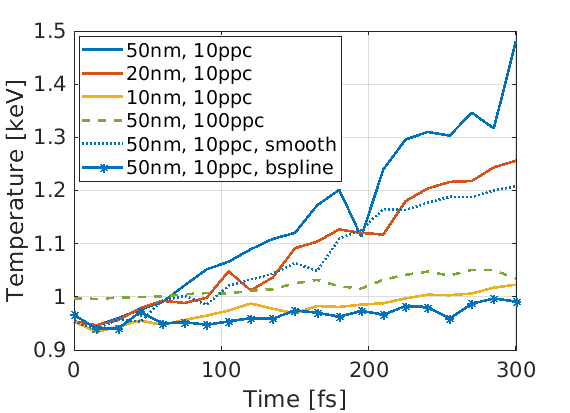
As there is no source of energy in this simulation, any temperature increase must be non-physical. Here we see that as cell-size decreases, or particles per cell increases, the self-heating is reduced. Switching on current smoothing, or switching to a higher order macro-particle shape (B-spline) also reduces self-heating. All these features come at a cost of a greater runtime, so it is up to the user to decide how much self-heating mitigation is required.