Lasers
EPOCH can support laser sources on the boundaries, with a wide array of spatial and temporal profiles. These examples provide basic input decks for simulating lasers in vacuum. General documentation on the EPOCH laser block can be found here.
Simple plane wave
This input deck provides the most basic form of laser. We use uniform spatial and temporal profiles, and inspect the Poynting flux in the simulation window. As a typical rule of thumb, allow 20 cells per wavelength to get a good resolution.
begin:control
    nx = 200
    ny = 400
    t_end = 100e-15
    x_min = 0
    x_max = 10e-6
    y_min = -10e-6
    y_max = 10e-6
    stdout_frequency = 100
end:control

begin:boundaries
    bc_x_min = simple_laser
    bc_x_max = open
    bc_y_min = open
    bc_y_max = open
end:boundaries

begin:laser
    boundary = x_min
    intensity_w_cm2 = 1.0e18
    lambda = 1.0e-6
end:laser

begin:output
    dt_snapshot = 10 * femto
    poynt_flux = always
end:output
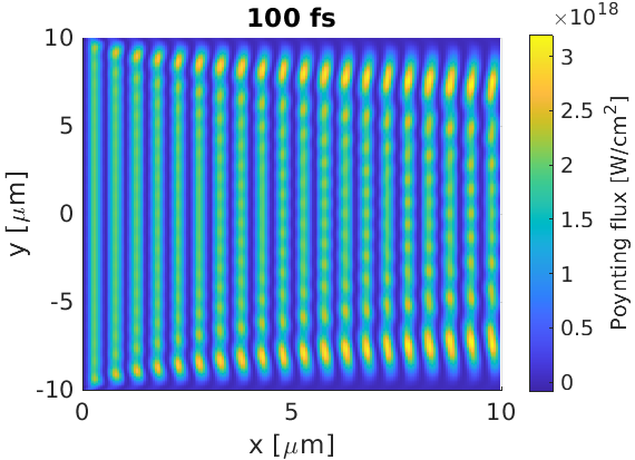
As we have specified a time-averaged intensity of $10^{18} \text{ Wcm}^{-2}$, we expect the Poytning flux to range 0 to $2\times 10^{18} \text{ Wcm}^{-2}$, which we can see here. Note that, because our laser profile reaches the $y_{min}$ and $y_{max}$ boundaries, some noise has been introduced here. In practice, these boundary effects are less of an issue, as simulations are expected to mainly deal with laser pulses.
Laser pulse
Using the maths parser, we can create a laser pulse which has a Gaussian profile in time and space for the intensity distribution, $I$:
$ I(y,t) \propto e^{-(y-y_0)^2/2\sigma_y^2} e^{-(t-t_0)^2/2\sigma_t^2}$
where we consider a 2D simulation with an $x$ propagating laser.
Let the full-width-at-half-maximum of the spatial and temporal profiles be 5 $\mu m$ and 40 fs respectively for the intensity $I$ distribution. The relationship between $\sigma$ and the $fwhm$ for a Gaussian distribution is:
$\sigma = \frac{fwhm}{2\sqrt{2 \ln(2)}}$
However, the profile keys in the laser block describe modifications to the boundary electric fields, $E$, and as $I \propto E^2$, the $E$ profile must satisfy
$ E(y,t) \propto e^{-((y-y_0)/2\sigma_y)^2} e^{-((t-t_0)/2\sigma_t)^2}$
The EPOCH
maths parser provides
a special gauss(x,x_0,w) command for use in the input.deck, which sets a
profile of the form:
$e^{-(x-x_0)^2/w^2}$
Hence, we may use this gauss function to model the electric field profiles if
we set
$w = \frac{fwhm}{\sqrt{2\ln(2)}}$
where $fwhm$ refers to the intensity distribution.
We can let the spatial profile peak at $y=0$. We don’t want the laser to peak at $t=0$, as this would ignore the rising intensity. Instead, let us start when the laser pulse is 10% of its maximum value - the half-width-at-10%-maximum, $hw0.1m$. For a Gaussian beam, this is:
$hw0.1m = \frac{fwhm}{2} \sqrt{\frac{\ln(10)}{\ln(2)}}$
begin:control
    nx = 700
    ny = 400
    t_end = 100e-15
    x_min = 0
    x_max = 35e-6
    y_min = -10e-6
    y_max = 10e-6
    stdout_frequency = 100
end:control

begin:boundaries
    bc_x_min = simple_laser
    bc_x_max = open
    bc_y_min = open
    bc_y_max = open
end:boundaries

begin:constant
    t_fwhm = 40.0e-15
    y_fwhm = 5.0e-6
    w_t = t_fwhm / sqrt(2*loge(2))
    w_y = y_fwhm / sqrt(2*loge(2))
    t_hw01m = 0.5 * t_fwhm * sqrt(loge(10)/loge(2))
end:constant

begin:laser
    boundary = x_min
    intensity_w_cm2 = 1.0e18
    lambda = 1.0e-6
    profile = gauss(y,0,w_y)
    t_profile = gauss(time,t_hw01m,w_t)
end:laser

begin:output
    dt_snapshot = 10 * femto
    poynt_flux = always
end:output
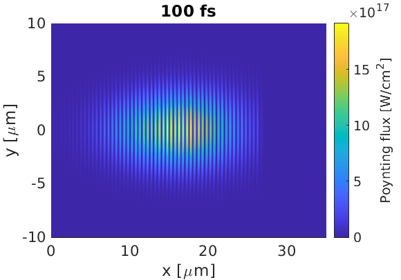
Here we see that the laser $fwhm$ in $x$ and $y$ are 12 $\mu m$ and 5 $\mu m$ respectively, where the $x$ $fwhm$ corresponds to a temporal FWHM of 40 fs, as expected. Also, because there is little contact between the pulse and the boundaries, we do not have any numerical boundary disturbance.
Angled laser pulse
A Gaussian laser pulse like the one in the previous example may be injected at
an angle into an EPOCH simulation. This is achieved by defining the spatial and
temporal laser envelopes in a rotated co-ordinate system (temporal envelope is
equivalent to an envelope in the laser-propagation direction). In this example,
the parameters y_rot and t_rot will describe the transverse and longitudinal
co-ordinates in the rotated co-ordinate system. Transformations are required
for both the profile and the phase of the laser.
EPOCH uses the provided intensity to set $B$ values parallel to the boundary -
on x_min, this sets $B_y$ and $B_z$. EPOCH sets these fields assuming the
laser travels perpendicular to the boundary, but this will over-estimate the $B$
fields in our rotated co-ordinate system, as part of the magnetic field will
also oscillate in the boundary normal direction. To correct for this, an
additional cos(theta) parameter is required for intensity in the laser
block.
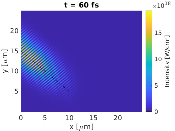
Finally, we must also be careful about the time when the peak laser intensity enters the simulation. In the previous example, we set this to the half-time at 10% maximum, such that the laser started at 10% of its maximum intensity and then increased to full. In a rotated laser, the wave-front corresponding to the peak intensity arrives earlier on one of the laser edges than the other. Let us set the injection time such that this “early edge” starts at 1% of the maximum intensity. We will define the $y$ position of this “early edge” to be the half-width at 1% maximum for the spatial profile. This way, we will sufficiently model the full envelope, regardless of the injection angle.
Here we provide an input deck which specifies a point on the laser path, and an injection angle. Two constant blocks are provided: the first is for users to set laser parameters, and the second derives parameters in the rotated co-ordinate system.
begin:control
  nx = 500
  ny = 500
  t_end = 200e-15
  x_min = 0
  x_max = 25e-6
  y_min = 0e-6
  y_max = 25e-6
  stdout_frequency = 50
end:control

begin:boundaries
  bc_x_min = simple_laser
  bc_x_max = open
  bc_y_min = open
  bc_y_max = open
end:boundaries

begin:constant
  t_fwhm = 40.0e-15          # Temporal FWHM
  y_fwhm = 5.0e-6            # Spatial FWHM
  y_foc = 5.0e-6             # y co-ord on laser path
  x_foc = 10.0e-6            # x co-ord on laser path
  las_theta_deg = -45        # Laser angle to boundary normal
  I_peak_Wcm2 = 1.0e19       # Peak cycle-averaged intensity
  las_lambda = 1.0e-6        # Laser wavelength
end:constant

begin:constant
  las_theta = las_theta_deg * pi / 180.

  y0 = y_foc - (x_foc - x_min) * tan(las_theta)
  y_rot = y*cos(las_theta)
  y0_rot = y0*cos(las_theta)
  w_y = y_fwhm / sqrt(2*loge(2))
  y_hw001m = 0.5 * y_fwhm * sqrt(loge(100)/loge(2)) # Half-width 1% max

  w_t = t_fwhm / sqrt(2*loge(2))
  t_hw001m = 0.5 * t_fwhm * sqrt(loge(100)/loge(2)) # Half-width 1% max
  t_rot = time - (y-y0)*sin(las_theta)/c
  t_hw001m_rot = t_hw001m + abs(y_hw001m * sin(las_theta) / c)

  I_peak_rot = I_peak_Wcm2 * cos(las_theta)
end:constant

begin:laser
  boundary = x_min
  intensity_w_cm2 = I_peak_rot
  lambda = las_lambda
  profile = gauss(y_rot, y0_rot, w_y) * gauss(t_rot, t_hw001m_rot, w_t)
  phase = -2 * pi * (y-y0_rot) * sin(las_theta) / las_lambda
end:laser

begin:output
  dt_snapshot = t_end / 10
  poynt_flux = always
end:output
Here, we see the Poynting flux corresponds to a rotated Gaussian pulse. The expected laser trajectory is marked with a dashed line for comparison. We see that the wavelength, along with the spatial and temporal FWHM are as expected.
Focussing a Gaussian Beam
A laser can be driven on the boundary so that it focusses on a given spot. Basic details of how to do this are here. To summarise, using the paraxial approximation, the electric fields for a $x$-propagating, $y$-polarised Gaussian beam take the form:
$\pmb{E}(r,x) = E_0 \frac{w_0}{w(x)} e^{-r^2/w(x)^2} e^{-i(kx + k\frac{r^2}{2R_c(x)}-\psi(x))} \hat{\pmb{y}}$
where
- $r$ is the radial distance from the laser propagation axis
- $x$ is axial distance along the wave, with $x=0$ at the focus
- $E_0$ is the peak electric field amplitude at the focus
- $w(x)$ is the beam-waist at $x$ (radial distance where field strength drops by $e^{-1}$)
- $w_0$ is $w(x=0)$
- $k$ is the laser wave-vector
- $R_c(x)$ is the radius of curvature at $x$
- $\psi(x)$ is the Gouy phase correction
If the fields on the simulation boundary are of this form, then the fields will propagate according to this equation, and a focal spot will be formed. Note that this propagation is only expected provided the paraxial approximation is satisfied. This implies that, for vacuum propagation, the laser wavelength, $\lambda$ is much smaller than the beam-waist: $\lambda « w_0$.
The following deck gives an example for a laser attached to x_min. Two constant blocks are provided: the first gives the user control over the focused laser properties, and the second derives variables to be used in the laser block. The user only needs to touch the first, which sets the intensity full-width-at-half-maximum (related to beam-waist), the peak, cycle-averaged intensity, the laser wave-length and the distance from the $x_{min}$ boundary to the focal point.
begin:control
  t_end = 70e-15
  nx = 1000
  ny = 500
  x_min = -5e-6
  x_max = 15e-6
  y_min = -5e-6
  y_max =  5e-6
  stdout_frequency = 100 # Print ETA
end:control

begin:boundaries
    bc_x_min = simple_laser
    bc_x_max = open
    bc_y_min = open
    bc_y_max = open
end:boundaries

begin:constant
  I_0_Wcm2 = 1e16 # Peak cycle-averaged intensity of the laser (Wcm^-2)
  I_0 = I_0_Wcm2 * 1e4
  lambda_L = 1e-6 # Wavelength of the laser
  r_fwhm_L = 2e-6 # Intensity fwhm in r
end:constant

begin:constant
  # Convert co-ordinates
  r = sqrt(y^2)# + z^2) # Change for 3D

  # Focusing distance
  x_foc = -x_min # Boundary to focal point distance

  # Phase
  k_L = 2 * pi / lambda_L # Laser wave number
  w_0 = r_fwhm_L / (sqrt(2*loge(2))) # Focused beam waist
  x_Rr = pi * w_0^2 / lambda_L # Rayleigh range
  r_c_bound = x_foc * (1 + (x_Rr/x_foc)^2) # Radius of curvature at the boundary
  psi_Gouy = atan(-x_foc/x_Rr) # Boundary phase Gouy shift

  # Spatial profile
  w_bound = w_0 * sqrt(1 + (x_foc/x_Rr)^2)
  I_bound = I_0 * (w_0 / w_bound)^1 # Intensity on the boundary
  # In 3D I_boundary should be changed to: I_bound * (w_0 / w_bound)^2
end:constant

begin:laser
  boundary = x_min
  intensity = I_bound
  lambda = lambda_L
  profile = gauss(r, 0, w_bound) # Spatial profile
  phase = k_L * (r^2 / (2 * r_c_bound)) - psi_Gouy # Phase
end:laser

begin:output
  name = normal
  grid = always
  dt_snapshot = 10e-15
  poynt_flux = always
end:output
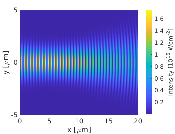
Note that the absolute maximum of the intensity is twice that of the peak cycle-averaged intensity because the laser is linearly polarised.
The deck is based on the laser test deck supplied with EPOCH, with a modified laser and longer runtime. Other classes of beam (Bessel etc) can be created similarly.