Injectors
It is possible to add macro-particles to the simulation window after the initial macro-particle load using the injector block. This can be done to simulate a particle beam passing through a boundary, or to replace macro-particles on the boundary of a flowing plasma volume. EPOCH provides support for two styles of injectors, one which is specified by plasma properties, and the other which reads particles from files.
Basic plasma injector
To demonstrate the basic injector syntax, we have created a simple example. Here
we inject macro-electrons through the x_min boundary, such that all electrons
have the same momentum, and the macro-particle weights are chosen to ensure the
injected density is $10^{10} \text{ m}^{-3}$. No macro-particles are initially
loaded into the simulation window.
begin:control
    nx = 500
    ny = 200
    t_end = 20.0e-15
    x_min = 0
    x_max = 25e-6
    y_min = -5e-6
    y_max = 5e-6
    stdout_frequency = 100
end:control

begin:boundaries
    bc_x_min = open
    bc_x_max = open
    bc_y_min = open
    bc_y_max = open
end:boundaries

begin:species
    name = Electron
    mass = 1.0
    charge = -1.0
end:species

begin:injector
   boundary = x_min
   species = Electron
   number_density = 1.0e10
   drift_x = 1.0e-20
   npart_per_cell = 10
end:injector

begin:output
    dt_snapshot = t_end
    number_density = always
end:output
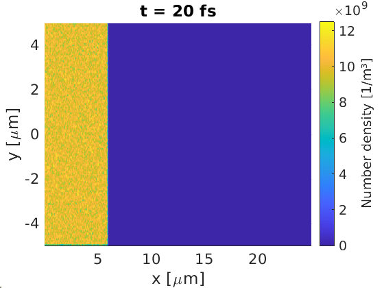
This figure shows macro-particles have been injected through the x_min
boundary,
with weights set to match the desired density.
Flowing plasma injector
If we set up a problem where a flowing plasma fills the simulation window, then the plasma will start to flow through a boundary after the initial load. As this happens, macro-particles will exit the simulation on one side, leaving a vacuum on the other side. If we added an injector to the vacuum side, then we can introduce a source of new macro-particles to replace the lost macro-particles. To do this, we can set the temperature and number density of the injector to match that of the initial plasma.
begin:control
    nx = 500
    ny = 200
    t_end = 20.0e-15
    x_min = 0
    x_max = 25e-6
    y_min = -5e-6
    y_max = 5e-6
    stdout_frequency = 100
end:control

begin:boundaries
    bc_x_min = open
    bc_x_max = open
    bc_y_min = open
    bc_y_max = open
end:boundaries

begin:species
    name = Electron
    mass = 1.0
    charge = -1.0
    npart = nx * ny * 10
    drift_x = 1.0e-20
    temp_ev = 1.0e3
    number_density = 1.0e10
end:species

begin:injector
   boundary = x_min
   species = Electron
   number_density = 1.0e10
   drift_x = 1.0e-20
   temp_ev = 1.0e3
   npart_per_cell = 10
end:injector

begin:output
    dt_snapshot = t_end
    number_density = always
end:output
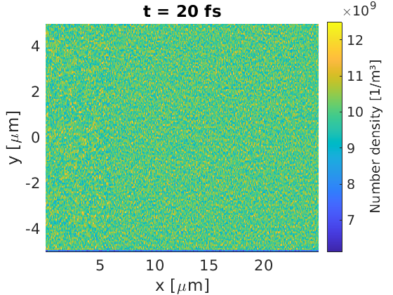
Here we see that the plasma density is still uniform, even though the plasma
is drifting towards x_max. Particles above $6\text{ }\mu\text{m}$ were loaded
at the start of the simulation, and those below have been replaced with
injectors. No sign of discontinuity on the injector/initial macro-particle
boundary is present.
Particle bunch injection
The profile of the injector can be modified to introduce spatial and temporal
variation, which would be useful for describing injected particle bunches.
We can set a Gaussian profile using the gauss(x,x0,w) function in the
maths parser, which represents
$e^{-(x-x_0)^2/w^2}$
In this formula, $w$ is related to the Gaussian full-width-at-half-maximum according to
$w = \frac{fwhm}{2\sqrt{\ln 2}}$
For the temporal profile, let us simulate the full-width-at-10%-maximum. This means the peak should arrive in the simulation at the half-width-at-10%-maximum time, given by
$hw0.1m = \frac{fwhm}{2} \sqrt{\frac{\ln(10)}{\ln(2)}}$
begin:control
    nx = 500
    ny = 200
    t_end = 20.0e-15
    x_min = 0
    x_max = 25e-6
    y_min = -5e-6
    y_max = 5e-6
    stdout_frequency = 100
end:control

begin:boundaries
    bc_x_min = open
    bc_x_max = open
    bc_y_min = open
    bc_y_max = open
end:boundaries

begin:species
    name = Electron
    mass = 1.0
    charge = -1.0
end:species

begin:constant
    x_fwhm = 1.0e-6
    y_fwhm = 1.0e-6
    t_fwhm = x_fwhm / c
    w_t = t_fwhm / (2.0 * sqrt(loge(2)))
    w_y = y_fwhm / (2.0 * sqrt(loge(2)))
    t_hw01m = 0.5 * t_fwhm * sqrt(loge(10) / loge(2))
end:constant

begin:injector
   boundary = x_min
   species = Electron
   number_density = 1.0e10 * gauss(y,0,w_y) * gauss(time,t_hw01m,w_t)
   number_density_min = 1.0e9
   t_start = 0
   t_end = 2.0 * t_hw01m
   drift_x = 1.0e-20
   temp_ev = 1.0e3
   npart_per_cell = 10
end:injector

begin:output
    dt_snapshot = t_end
    number_density = always
end:output
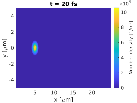
The injected pulse is seen to have the desired properties. Note that we have introduced a threshold density for macro-particle injection with
number_density_min = 1.0e9
This line ensures that profiled densities below this value will not load macro-particles into the simulation. This prevents the code from loading too many low-weight macro-particles which would slow down the code.
File injectors
If the in-built density, temperature and drift do not provide the desired injection behaviour, or if you’re trying to inject specific particles from a different simulation, then you may find file-injectors useful. Here the user can specify the injection time, position and momentum of each injected macro-particle from file. Unlike other file-packages in EPOCH, the file-injectors read from simple text files.
For this simple example, let us inject a macro-electron of weight 10 into a
2D simulation window each femtosecond. The momenta of these macro-particles will
be set such that they are highly relativistic, with a speed close to $c$. To
check if they have been injected correctly, let us insert a particle probe
one micron from the injection boundary. Let us also use the -DPROBE_TIME
compiler flag to see the exact time macro-particles pass the probe. See the
section on
compiler flags
for help with switching on the probe-time capability.
We need to use separate files for each macro-particle variable, and particles must be listed in chronological order of injection. For this demonstration, the files contain:
inject_t.txt
1.0e-15
2.0e-15
3.0e-15
4.0e-15
5.0e-15
6.0e-15
7.0e-15
8.0e-15
9.0e-15
10.0e-15
inject_w.txt
10
10
10
10
10
10
10
10
10
10
inject_y.txt
0
0
0
0
0
0
0
0
0
0
inject_px.txt
1.0e-20
1.0e-20
1.0e-20
1.0e-20
1.0e-20
1.0e-20
1.0e-20
1.0e-20
1.0e-20
1.0e-20
and the input.deck reads:
begin:control
    nx = 500
    ny = 200
    t_end = 20.0e-15
    x_min = 0
    x_max = 25e-6
    y_min = -5e-6
    y_max = 5e-6
    stdout_frequency = 100
end:control

begin:boundaries
    bc_x_min = open
    bc_x_max = open
    bc_y_min = open
    bc_y_max = open
end:boundaries

begin:species
    name = Electron
    mass = 1.0
    charge = -1.0
end:species

begin:injector
    boundary = x_min
    species = Electron
    inject_from_file = T
    y_data = "inject_y.txt"
    px_data = "inject_px.txt"
    w_data = "inject_w.txt"
    t_data = "inject_t.txt"
end:injector

begin:output
    dt_snapshot = t_end
    particle_probes = always
end:output

begin:probe
   name = Electron_probe
   point = (1.0e-6, 0.0)
   normal = (1.0, 0.0)
   ek_min = 0.0
   ek_max = -1.0
   include_species:Electron
   dumpmask = always
end:probe
For injector files, the code will look in the same directory as the input.deck
file. The full path is not required like in other file-reading blocks. If we
open 0001.sdf (possibly using the GetDataSDF.m function in
epoch/SDF/Matlab), we see the times each macro-particle passes the probe. We
can label each macro-particle by its line in the injector files, and we can
obtain a probe-time vs file-line plot
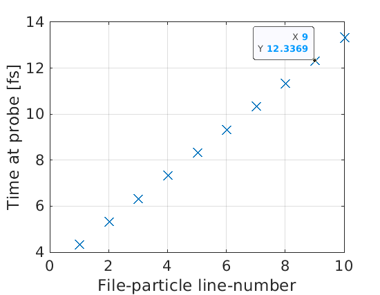
Due to the position of the probe, and the speed of the macro-particles, we expect these probe times to be 3.337 fs after the particle injection time. This matches the behaviour seen in the probe data, which shows that the file injectors are working as intended.