IDL or GDL
Using IDL to visualise data
The EPOCH distribution comes with procedures for loading and inspecting
SDF self-describing data files. The IDL routines are held in the
SDF/IDL/ directory. There is also a procedure named
Start.pro in each of the epoch\*d/ directories
which is used to set up the IDL environment.
To load data into IDL, navigate to one of the base directories (eg.
epoch/epoch2d/ where epoch/ is the directory in which you have
checked out the git repository) and type the following:
$> idl Start.pro
IDL Version 8.1 (linux x86_64 m64). (c) 2011, ITT Visual Information Solutions
Installation number: .
+Licensed for use by: STAR404570-5University of Warwick
.
% Compiled module: TRACKEX_EVENT.
% Compiled module: ISOPLOT.
% Compiled module: READVAR.
% Compiled module: LOADSDFFILE.
% Compiled module: SDFHANDLEBLOCK.
% Compiled module: SDFGETPLAINMESH.
% Compiled module: SDFGETLAGRANMESH.
% Compiled module: SDFGETPOINTMESH.
% Compiled module: SDFGETPLAINVAR.
% Compiled module: SDFGETPOINTVAR.
% Compiled module: SDFGETCONSTANT.
% Compiled module: SDFCHECKNAME.
% Compiled module: INIT_SDFHELP.
% Compiled module: GETDATA.
% Compiled module: GETSTRUCT.
% Compiled module: EXPLORE_DATA.
% Compiled module: EXPLORE_STRUCT.
% Compiled module: LIST_VARIABLES.
% Compiled module: QUICK_VIEW.
% Compiled module: GET_WKDIR.
% Compiled module: SET_WKDIR.
% Compiled module: INIT_STARTPIC.
% Compiled module: INIT_WIDGET.
% Compiled module: GENERATE_FILENAME.
% Compiled module: COUNT_FILES.
% Compiled module: LOAD_RAW.
% Compiled module: GET_SDF_METATEXT.
% Compiled module: VIEWER_EVENT_HANDLER.
% Compiled module: EXPLORER_EVENT_HANDLER.
% Compiled module: XLOADCT_CALLBACK.
% Compiled module: LOAD_DATA.
% Compiled module: DRAW_IMAGE.
% Compiled module: LOAD_META_AND_POPULATE_SDF.
% Compiled module: CLEAR_DRAW_SURFACE.
% Compiled module: SDF_EXPLORER.
% Compiled module: EXPLORER_LOAD_NEW_FILE.
% Compiled module: CREATE_SDF_VISUALIZER.
% Compiled module: VIEWER_LOAD_NEW_FILE.
% LOADCT: Loading table RED TEMPERATURE
IDL>
This starts up the IDL interpreter and loads in all of the libraries for loading and inspecting SDF files.
We begin by inspecting SDF file contents and finding out what variables it contains. To do this we execute the list variables procedure call which is provided by the EPOCH IDL library.
At each timestep for which EPOCH is instructed to dump a set of variables a new data file is created. These files take the form 0000.sdf. For each new dump the number is incremented. The procedure call accepts up to two arguments. The first argument is mandatory and specifies the number of the SDF file to be read in. This argument can be any integer from 0 to 9999. It is padded with zeros and the suffix ‘.sdf’ appended to the end to give the name of the data file. eg. 99 ⇒ ‘0099.sdf’. The next arguments is optional. The keyword wkdir specifies the directory in which the data files are located. If this argument is omitted then the currently defined global default is used. Initially, this takes the value Data but this can be changed using the set_wkdir procedure and queried using the get_wkdir() function.
IDL> list_variables,0,"Data"
Available elements are
1) EX (ELECTRIC_FIELD) : 2D Plain variable
2) EY (ELECTRIC_FIELD) : 2D Plain variable
3) EZ (ELECTRIC_FIELD) : 2D Plain variable
4) BX (MAGNETIC_FIELD) : 2D Plain variable
5) BY (MAGNETIC_FIELD) : 2D Plain variable
6) BZ (MAGNETIC_FIELD) : 2D Plain variable
7) JX (CURRENT) : 2D Plain variable
8) JY (CURRENT) : 2D Plain variable
9) JZ (CURRENT) : 2D Plain variable
10) WEIGHT_ELECTRON (PARTICLES) : 1D Point variable
11) WEIGHT_PROTON (PARTICLES) : 1D Point variable
12) PX_ELECTRON (PARTICLES) : 1D Point variable
13) PX_PROTON (PARTICLES) : 1D Point variable
14) GRID_ELECTRON (GRID) : 2D Point mesh
15) GRID_PROTON (GRID) : 2D Point mesh
16) EKBAR (DERIVED) : 2D Plain variable
17) EKBAR_ELECTRON (DERIVED) : 2D Plain variable
18) EKBAR_PROTON (DERIVED) : 2D Plain variable
19) CHARGE_DENSITY (DERIVED) : 2D Plain variable
20) NUMBER_DENSITY (DERIVED) : 2D Plain variable
21) NUMBER_DENSITY_ELECTRON (DERIVED) : 2D Plain variable
22) NUMBER_DENSITY_PROTON (DERIVED) : 2D Plain variable
23) GRID (GRID) : 2D Plain mesh
24) GRID_EN_ELECTRON (GRID) : 1D Plain mesh
25) EN_ELECTRON (DIST_FN) : 3D Plain variable
26) GRID_X_EN_ELECTRON (GRID) : 2D Plain mesh
27) X_EN_ELECTRON (DIST_FN) : 3D Plain variable
28) GRID_X_PX_ELECTRON (GRID) : 2D Plain mesh
29) X_PX_ELECTRON (DIST_FN) : 3D Plain variable
IDL>
Each variable in the SDF self-describing file format is assigned a name and a class as well as being defined by a given variable type. The “list_variables” procedure prints out the variable name followed by the variable’s class in parenthesis. Following the colon is a description of the variable type.
To retrieve the data, you must use the getdata() function call. The function must be passed a snapshot number, either as the first argument or as a keyword parameter “snapshot”. It also accepts the wkdir as either the second argument or the keyword parameter “wkdir”. If it is omitted altogether, the current global default is used. Finally, it accepts a list of variables or class of variables to load. Since it is a function, the result must be assigned to a variable. The object returned is an IDL data structure containing a list of named variables.
To load either a specific variable or a class of variables, specify the name prefixed by a forward slash. It should be noted here that the IDL scripting language is not case sensitive so $P_x$ can be specified as either “/Px” or “/px”.
We will now load and inspect the “Grid” class, this time omitting the optional “wkdir” parameter. This time we will load from the third dump file generated by the EPOCH run, which is found in the file 0002.sdf since the dump files are numbered starting from zero.
Inspecting Data
IDL> gridclass = getdata(1,/grid)

IDL> help,gridclass,/structures
** Structure <22806408>, 11 tags, length=536825024, data length=536825016, refs=1:
   FILENAME        STRING    'Data/0001.sdf'
   TIMESTEP        LONG                43
   TIME            DOUBLE       5.0705572e-15
   GRID_ELECTRON   STRUCT    -> <Anonymous> Array[1]
   GRID_PROTON     STRUCT    -> <Anonymous> Array[1]
   GRID            STRUCT    -> <Anonymous> Array[1]
   X               DOUBLE    Array[1024]
   Y               DOUBLE    Array[512]
   GRID_EN_ELECTRON
                   STRUCT    -> <Anonymous> Array[1]
   GRID_X_EN_ELECTRON
                   STRUCT    -> <Anonymous> Array[1]
   GRID_X_PX_ELECTRON
                   STRUCT    -> <Anonymous> Array[1]
IDL> help,gridclass.grid,/structures
** Structure <1701168>, 5 tags, length=12376, data length=12376, refs=2:
   X               DOUBLE    Array[1025]
   Y               DOUBLE    Array[513]
   LABELS          STRING    Array[2]
   UNITS           STRING    Array[2]
   NPTS            LONG      Array[2]
Here we have used IDL’s built in “help” routine and passed the “/structures” keyword which prints information about a structure’s contents rather than just the structure itself.
Since “Grid” is a class name, all variables of that class have been loaded into the returned data structure. It is a nested type so many of the variables returned are structures themselves and those variables may contain structures of their own.
The “Grid” variable itself contains x" and “y” arrays containing the $x$ and $y$ coordinates of the 2D cartesian grid. The other variables in “Grid” the structure are metadata used to identify the type and properties of the variable. In order to access the “Grid” variable contained within the “gridclass” data structure we have used the “.” operator. In a similar way, we would access the “x” array contained within the “Grid” variable using the identifier “gridclass.grid.x”.
Getting Help in IDL
IDL is a fairly sophisticated scripting environment with a large library of tools for manipulating data. Fortunately, it comes with a fairly comprehensive array of documentation. This can be accessed by typing ? at the IDL prompt.
IDL> ?
% ONLINE_HELP: Starting the online help browser.
IDL>
The documentation is divided into books aimed at users or developers and is fully searchable and cross indexed.
Manipulating And Plotting Data
Once the data has been loaded from the SDF file we will want to extract the specific data we wish to analyse, perhaps perform some mathematical operations on it and then plot the results.
To do this we must learn a few basic essentials about the IDL scripting language. Since we are all familiar with the basic concepts shared by all computer programming languages, I will just provide a brief overview of the essentials and leave other details to the excellent on-line documentation.
IDL supports multidimensional arrays similar to those found in the FORTRAN programming language. Whole array operations are supported such as “5*array” to multiply every element of “array” by 5. Also matrix operations such as addition and multiplication are supported.
The preferred method for indexing arrays is to use brackets. It is possible to use parenthesis instead but this usage is deprecated. Column ordering is the same as that used by FORTRAN, so to access the $(i,j,k)$th element of an array you would use “array[i,j,k]”. IDL arrays also support ranges so “array[5:10,3,4]” will return a one dimensional array with five elements. “array[5:*]” specifies elements five to $n$ of an $n$ element array. “array[*,3]” picks out the third row of an array.
There are also a wide range of routines for querying and transforming arrays of data. For example, finding minimum and maximum values, performing FFTs, etc. These details can all be found by searching the on-line documentation.
Finally, IDL is a full programming language so you can write your own functions and procedures for processing the data to suit your needs.
1D Plotting in IDL
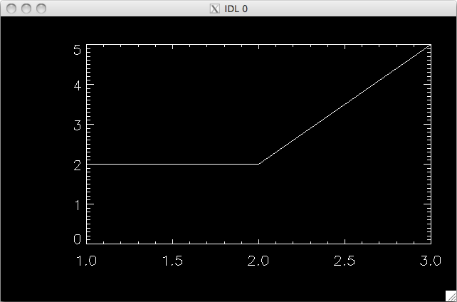
The most commonly performed plot and perhaps the most useful data analysis tool is the 1D plot. In IDL, this is performed by issuing the command plot,x,y where “x” and “y” are one dimensional arrays of equal length. For each element “x[i]” plotted on the $x$-axis the corresponding value “y[i]” is plotted along the $y$-axis. As a simple example:
IDL> plot,[1,2,3],[2,2,5]
Gives rise to the following plot:
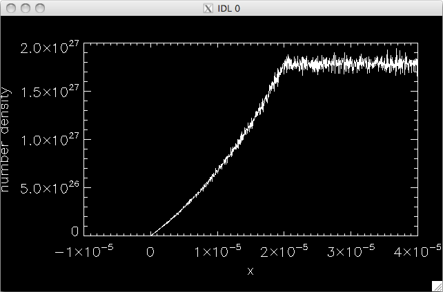
As a more concrete example, we will now take a one-dimensional slice through the 2D array “Number Density” read in from our SDF data file. In this example we will give the $x$ and $y$ axes labels by passing extra parameters to the “plot” routine. A full list of parameters can be found in the on-line documentation. In this example we also make use of the “$” symbol which is IDL’s line continuation character.
IDL> data = getdata(0)
IDL> plot,data.x,data.number_density[*,256],xtitle='x', $
IDL>    ytitle='number density'
This command generates the following plot:
Postscript Plots
The plots shown so far have just been screen-shots of the interactive IDL plotting window. These are fairly low quality and could included as figures in a paper.
In order to generate publication quality plots, we must output to the postscript device. IDL maintains a graphics context which is set using set plot the command. The two most commonly used output devices are “x” which denotes the X-server and “ps” which is the postscript device. Once the desired device has been selected, various attributes of its behaviour can be altered using the device procedure. For example, we can set the output file to use for the postscript plot. By default, a file with the name “idl.ps” is used.
Note that this file is not fully written until the postscript device is closed using the device,/close command. When we have finished our plot we can resume plotting to screen by setting the device back to “x”.
IDL> set_plot,'ps'
IDL> device,filename='out.ps'
IDL> plot,data.x,data.number_density[*,256],xtitle='x', $
IDL>    ytitle='number density',charsize=1.5
IDL> device,/close
IDL> set_plot,'x'
This set of commands results in the following plot being written to a file named “out.ps”.

By default, IDL draws its own set of fonts called “Hershey vector fonts”. Much better looking results can be obtained by using a postscript font instead. These options are passed as parameters to the device procedure. More details can be found in the on-line documentation under “Reference Guides $\Rightarrow$ IDL Reference Guide $\Rightarrow$ Appendices $\Rightarrow$ Fonts”.
Contour Plots in IDL
Whilst 1D plots are excellent tools for quantitive analysis of data, we can often get a better qualitative overview of the data using 2D or 3D plots.
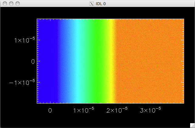
One commonly used plot for 2D is the contour plot. The aptly named contour,z,x,y procedure takes a 2D array of data values, “z”, and plots them against $x$ and $y$ axes which are specified in the 1D “x” and “y” arrays. The number of contour lines to plot is specified by the “nlevels” parameter. If the “/fill” parameter is used then IDL will fill each contour level with a solid colour rather than just drawing a line at the contour value.
The example given below plots a huge number of levels so that a smooth looking plot is produced. “xstyle=1” requests that the $x$ axes drawn exactly matches the data in the variable rather than just using a nearby rounded value and similarly for “ystyle=1”.
IDL> n=100
IDL> levels=max(data.number_density)*findgen(n)/(n-1)
IDL> colors=253.*findgen(n)/(n-1)+1
IDL> contour,data.number_density,data.x,data.y,xstyle=1,ystyle=1, $
IDL>    levels=levels,/fill,c_colors=colors
Issuing these commands gives us the contour plot shown below. Note that the colour table used is not the default one but has been constructed to be similar to the one used by VisIt.
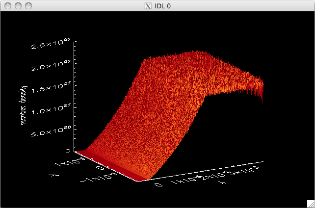
Shaded Surface Plots in IDL
Another method for visualising 2D datasets is to produce a 3D plot in which the data is elevated in the $z$ direction by a height proportional to its value. IDL has two versions of the surface plot. surface produces a wireframe plot and shade surf produces a filled and shaded one. As we can see from the following example, many of IDL’s plotting routines accept the same parameters and keywords.
The first command shown here, loadct,3, asks IDL to load the third colour table which is"RED_TEMPERATURE".
IDL> loadct,3
IDL> shade_surf,data.number_density,data.x,data.y,xstyle=1, $
IDL>    ystyle=1,xtitle='x',ytitle='y',ztitle='number density',charsize=3
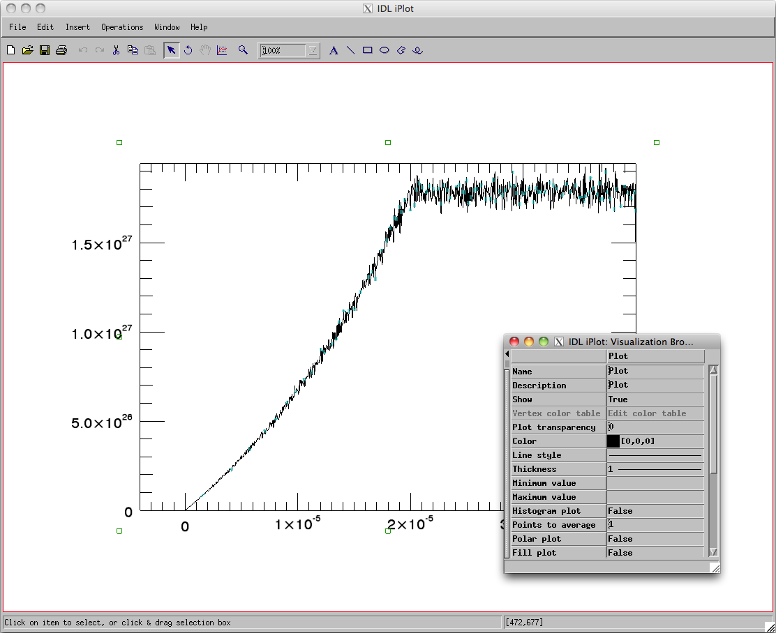
Interactive Plotting
Finally, in recent versions of IDL (not GDL) it is now possible to perform all of these plot types in an interactive graphical user interface. The corresponding procedures are launched with the commands iplot, icontour and isurface.
IDL> iplot,data.x,data.number_density[*,256]
IDL is an extremely useful tool but it also comes with a fairly hefty price tag. If you are not part of an organisation that will buy it for you then you may wish to look into a free alternative. It is also a proprietary tool and you may not wish to work within the restrictions that this imposes.
There are a number of free tools available which offer similar functionality to that of IDL, occasionally producing superior results.
For a simple drop-in replacement, the GDL project aims to be fully
compatible and works with the existing EPOCH IDL libraries after a
couple of small changes. Other tools worth investigating are
"yorick" and "python" with the
"SciPy" libraries. The python SDF reader documentation
will be added soon. At present there is no SDF reader for yorick but one
may be developed if there is sufficient demand.