BEAM

BEAM (Broad EPOCH Analysis Modules) is a collection of independent yet complementary open-source tools for analysing EPOCH simulations in Python, designed to be modular so researchers can adopt only the components they require without being constrained by a rigid framework. In line with the FAIR principles — Findable, Accessible, Interoperable, and Reusable — each package is openly published with clear documentation and versioning (Findable), distributed via public repositories (Accessible), designed to follow common standards for data structures and interfaces (Interoperable), and includes licensing and metadata to support long-term use and adaptation (Reusable). The packages are as follows:

• sdf-xarray: Reading and processing SDF files and converting them to xarray.
• epydeck: Input deck reader and writer.
• epyscan: Create campaigns over a given parameter space using various sampling methods.

Originally developed by Joel Adams and the PlasmaFAIR Team at the York Plasma Institute under the EPSRC Grant EP/V051822/1.

Installation

All of the packages are available on PyPI and can be installed using pip:

pip install sdf-xarray epydeck epyscan

Each package can be used independently or together depending on your needs.

Citing

If any of the BEAM contribute to a project that leads to publication, please acknowledge this by citing the module in question. This can be done by clicking the “cite this repository” button located near the top right of their respective github pages.

sdf-xarray: analysing EPOCH output

sdf-xarray is a lightweight wrapper that reads EPOCH’s SDF files into xarray.Dataset objects. This provides:

• Lazy loading and memory-efficient handling of large datasets
• Easy slicing and plotting using matplotlib, xarray.plot, or hvplot
• Automatic normalisation of grid and variable names
• Integration with Jupyter notebooks and Dask for parallel analysis

The key features for this module are highlighted below, for in-depth documentation please visit https://sdf-xarray.readthedocs.io

Single file loading

import xarray as xr

ds = xr.open_dataset("0010.sdf")

ds["Electric_Field_Ex"]

# <xarray.DataArray 'Electric_Field_Ex' (X_x_px_deltaf_electron_beam: 16)> Size: 128B
# [16 values with dtype=float64]
# Coordinates:
#   * X_x_px_deltaf_electron_beam  (X_x_px_deltaf_electron_beam) float64 128B 1...
# Attributes:
#     units:    V/m
#     full_name: "Electric Field/Ex"

Multi file loading

To open a whole simulation at once, pass preprocess=sdf_xarray.SDFPreprocess() to xarray.open_mfdataset:

import xarray as xr
from sdf_xarray import SDFPreprocess

ds = xr.open_mfdataset("*.sdf", preprocess=SDFPreprocess())

print(ds)

# Dimensions:
# time: 301, X_Grid_mid: 128, ...
# Coordinates: (9) ...
# Data variables: (18) ...
# Indexes: (9) ...
# Attributes: (22) ...

SDFPreprocess checks that all the files are from the same simulation, as ensures there’s a time dimension so the files are correctly concatenated.

If your simulation has multiple output blocks so that not all variables are output at every time step, then those variables will have NaN values at the corresponding time points.

After having loaded in a series of datasets we can select a simulation file by calling the .isel() function where we pass in the parameter of time=0 where 0 can be a number between 0 and the total number of simulation files.

We can also use the .sel() function if we know the exact simulation time we want to select. There must be a corresponding dataset with this time for it work correctly.

print(f"There are a total of {ds["time"].size} time steps. (This is the same as the number of SDF files in the folder)")
# There are a total of 41 time steps. (This is the same as the number of SDF files in the folder)

print(f"The time steps are: {ds["time"].values}")
# The time steps are: [2.60596949e-17 5.00346143e-15 1.00069229e-14, ..., 2.00034218e-13]

sim_time = ds['time'].isel(time=20).values
print(f"The time at the 20th simulation step is {sim_time:.2e} s")
# The time at the 20th simulation step is 1.00e-13 s

ds["Electric_Field_Ex"].isel(time=20)
# OR
# ds["Electric_Field_Ex"].sel(time=sim_time)

Plotting

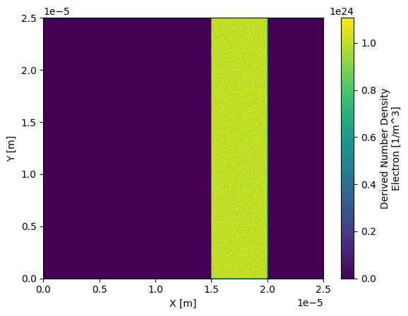
Since this package converts SDF files to xarray we can leverage the plotting features that are included in xarray. For example we can load in a SDF file and plot the number density of the electrons:

import xarray as xr

ds = xr.open_dataset("0010.sdf")

# NOTE: EPOCH saves the x and y axes into SDF files in the inverse order to that expected by xarray so we have to specify which axes is which otherwise our plot comes out inverted
ds["Derived_Number_Density_Electron"].plot(x="X_Grid_mid", y="Y_Grid_mid")

epydeck: Writing input deck files with Python

Writing large numbers of EPOCH input files by hand can be tedious and error-prone. epydeck (short for EPOCH Python deck) allows you to create and manipulate input decks in Python:

• Build decks using standard Python data structures
• Load, modify, and save EPOCH-style .deck files
• Designed to preserve comments and formatting where possible

The interface follows the standard Python json module:

• epydeck.load to read from a file object
• epydeck.loads to read from an existing string
• epydeck.dump to write to a file object
• epydeck.dumps to write to a string

The key features for this module are highlighted below, for in-depth documentation please visit, for in-depth documentation please visit https://github.com/epochpic/epydeck

Example

import epydeck

# Read from a file with `epydeck.load`
with open(filename) as f:
    deck = epydeck.load(f)

print(deck.keys())
# dict_keys(['control', 'boundaries', 'constant', 'species', 'laser', 'output_global', 'output', 'dist_fn'])

# Modify the deck as a usual python dict:
deck["species"]["proton"]["charge"] = 2.0

# Write to file
with open(filename, "w") as f:
    epydeck.dump(deck, f)

print(epydeck.dumps(deck))
# ...
# begin:species
#   name = proton
#   charge = 2.0
#   mass = 1836.2
#   fraction = 0.5
#   number_density = if((r gt ri) and (r lt ro), den_cone, 0.0)
#   number_density = if((x gt xi) and (x lt xo) and (r lt ri), den_cone, number_density(proton))
#   number_density = if(x gt xo, 0.0, number_density(proton))
# end:species
# ...

epyscan: Campaign generation and parameter sampling

epyscan (short for EPOCH Python scan) generates EPOCH campaigns over a parameter space using different sampling methods. It supports the following features:

• Defining scans over one or more input variables
• Support for grid and Latin hypercube sampling methods

Parameter space to be sampled is described by a dict where keys should be in the form of block_name:parameter, and values should be dicts with the following keys:

• "min": minimum value of the parameter
• "max": maximum value of the parameter
• "log": (optional) bool, if True then grid is done in log space for this parameter

The key features for this module are highlighted below, for in-depth documentation please visit, for in-depth documentation please visit https://github.com/epochpic/epyscan

Example

import pathlib
import epyscan
import epydeck

# Define the parameter space to be sampled. Here, we are varying the intensity
# and density
parameters = {
  # Intensity varies logarithmically between 1.0e22 and 1.0e24
  "constant:intens": {"min": 1.0e22, "max": 1.0e24, "log": True},
  # Density varies logarithmically between 1.0e20 and 1.0e24
  "constant:nel": {"min": 1.0e20, "max": 1e24, "log": True},
}

# Load a deck file to use as a template for the simulations
with open("template_deck_filename") as f:
  deck = epydeck.load(f)

# Create a grid scan object that will generate 4 different sets of parameters 
# within the specified ranges
grid_scan = epyscan.GridScan(parameters, n_samples=4)

# Define the root directory where the simulation folders will be saved. 
# This directory will be created if it doesn't exist
run_root = pathlib.Path("example_campaign")

# Initialize a campaign object with the template deck and the root directory. 
# This will manage the creation of simulation cases
campaign = epyscan.Campaign(deck, run_root)

# Generate the folders and deck files for each set of parameters in the
# grid scan
paths = [campaign.setup_case(sample) for sample in grid_scan]

# Save the paths of the generated simulation folders to a file
with open("paths.txt", "w") as f:
  [f.write(f"{path}\n") for path in paths]

# Opening paths.txt
# example_campaign/run_0_1000000/run_0_10000/run_0_100/run_0
# example_campaign/run_0_1000000/run_0_10000/run_0_100/run_1
# example_campaign/run_0_1000000/run_0_10000/run_0_100/run_2
# ...