Laser block
This block contains information about laser boundary sources. See EPOCH input deck for more information on the input deck.
Laser blocks attach an EM wave source to a boundary which is set as simple_laser.
begin:laser
   boundary = x_min
   id = 1
   intensity_w_cm2 = 1.0e15
   lambda = 1.06 * micron
   pol_angle = 0.0
   phase = 0.0
   t_profile = gauss(time, 40.0e-15, 40.0e-15)
   t_start = 0.0
   t_end = 80.0e-15
end:laser
As already mentioned in the discussion of laser boundaries in the boundaries block, lasers are attached to compatible boundaries here in the initial conditions deck.
boundary- The boundary on which to attach the laser. In 1D, the directions can be either x_min or x_max. “left” and “right” are accepted as a synonyms. In 2D, y_min and y_max may also be specified. These have synonyms of “down” and “up”. Finally, 3D adds z_min and z_max with synonyms of “back” and “front”.amp- The amplitude of the $E$ field of the laser in $V/m$.intensity- The intensity of the laser in $W/m^2$. There is no need to specify both intensity and amp and the last specified in the block is the value used. It is mandatory to specify at least one. The amplitude of the laser is calculated from intensity using the formulaamp = sqrt(2*intensity/c/epsilon0). “irradiance” is accepted as a synonym. Note that spatial and temporal profiles are applied to the electromagnetic fields of the laser, not the intensity. For example, if a laser enters through a boundary in a cell where the profile is set to 0.5, the intensity would be reduced to 0.25 the value set here.intensity_w_cm2- This is identical to the intensity parameter described above, except that the units are specified in $W/cm^2$.id- An id code for the laser. Used if you specify the laser time profile in the EPOCH source rather than in the input deck. Does not have to be unique, but all lasers with the same id will have the same time profile. This parameter is optional and is not used under normal conditions.omega- Angular frequency (rad/s not Hz) for the laser.frequency- Ordinary frequency (Hz not rad/s) for the laser.lambda- Wavelength in a vacuum for the laser specified in $m$. If you want to specify in $\mu m$ then you can multiply by the constant “micron”. One of lambda or omega (or frequency) is a required parameter.pol_angle- Polarisation angle for the electric field of the laser in radians. This parameter is optional and has a value of zero by default. The angle is measured with respect to the right-hand triad of propagation direction, electric and magnetic fields. Although the 1D code has no $y$ or $z$ spatial axis, the fields still have $y$ and $z$ components. If the laser is on x_min then the default $E$ field is in the $y$-direction and the $B$ field is the $z$-direction. The polarisation angle is measured clockwise about the $x$-axis with zero along the $E_y$ direction. If the laser is on x_max then the angle is anti-clockwise. **Similarly, for propagation directions: **y_min - angle about $y$-axis, zero along $z$-axis **z_min - angle about $z$-axis, zero along $x$-axis **y_max - angle anti-clockwise about $y$-axis, zero along $z$-axis **z_max - angle anti-clockwise about $z$-axis, zero along $x$-axispol- This is identical to pol_angle with the angle specified in degrees rather than radians. If both are specified then the last one is used.phase- The phase profile of the laser wavefront given in radians. Phase may be a function of both space and time. The laser is driven using ${\rm{sin}}(\omega t + \phi)$ and phase is the $\phi$ parameter. There is zero phase shift applied by default.profile- The spatial profile of the laser. This should be a spatial function not including any values in the direction normal to the boundary on which the laser is attached, and the expression will be evaluated at the boundary. It may also be time-dependant. The laser field is multiplied by the profile to give its final amplitude so the intention is to use a value between zero and one. By default it is a unit constant and therefore has no affect on the laser amplitude. This parameter is redundant in 1D and is only included for consistency with 2D and 3D versions of the code.t_profile- Used to specify the time profile for the laser amplitude. Like profile the laser field is multiplied by this parameter but it is only a function of time and not space. In a similar manner to profile, it is best to use a value between zero and one. Setting values greater than one is possible but will cause the maximum laser intensity to grow beyond amp. In previous versions of EPOCH, the profile parameter was only a function of space and this parameter was used to impose time-dependance. Since profile can now vary in time, t_profile is no longer needed but it has been kept to facilitate backwards compatibility. It can also make input decks clearer if the time dependance is given separately. The default value of t_profile is just the real constant value of 1.0.t_start- Start time for the laser in seconds. Can be set to the string “start” to start at the beginning of the simulation. This is the default value. When using this parameter, the laser start is hard. To get a soft start use the t_profile parameter to ramp the laser up to full strength.t_end- End time for the laser in seconds, can be set to the string “end” to end at the end of the simulation. This is the default value. When using this parameter, the laser end is clipped straight to zero at $t > t_end$. To get a soft end use the t_profile parameter to ramp the laser down to zero. If you add multiple laser blocks to the initial conditions file then the multiple lasers will be additively combined on the boundary.
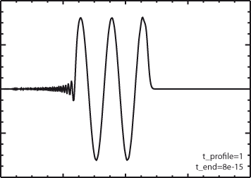
In theory, any laser time profile required is possible, but the core FDTD solver for the EM fields in EPOCH produces spurious results if sudden changes in the field intensity occur. This is shown below. The pulse shown on the left used a constant t_profile and used t_end to stop the laser after 8fs. Since the stopping time was not an exact multiple of the period, the result was to introduce spurious oscillations behind the pulse. If the laser had a finite phase shift so that the amplitude did not start at zero, a similar effect would be observed on the front of the pulse.
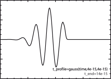
The second figure instead used a Gaussian window function with a characteristic width of 8fs as well as using t_end to introduce a hard cutoff. It can clearly be seen that there are no spurious oscillations and the wave packet propagates correctly, showing only some dispersive features.
There is no hard and fast rule as to how rapid the rise or fall for a laser can be, and the best advice is to simply test the problem and see whether any problems occur. If they do then there are various solutions. Essentially, the timestep must be reduced to the point where the sharp change in amplitude can be accommodated. The best solution for this is to increase the spatial resolution (with a comparable increase in the number of pseudoparticles), thus causing the timestep to drop via the CFL condition.
This is computationally expensive, and so a cheaper option is simply to decrease the input.deck option dt_multiplier. This artificially decreases the timestep below the timestep calculated from the internal stability criteria and allows the resolution of sharp temporal gradients. This is an inferior solution since the FDTD scheme has increased error as the timestep is reduced from that for EM waves. EPOCH includes a high order field solver to attempt to reduce this.