The control block contains information about the general code setup. See EPOCH input deck for more information on the input deck.

Basics

The block sets up the basic code properties for the domain, the end time of the code, the load balancer and the types of initial conditions to use.

The control block of a valid input deck for EPOCH2D reads as follows:

begin:control
   # Global number of gridpoints
   nx = 512 # in x
   ny = 512 # in y
   # Global number of particles
   npart = 10 * nx * ny

   # Final time of simulation
   t_end = 1.0e-12
   # nsteps = -1

   # Size of domain
   x_min = -0.1e-6
   x_max = 400.0e-6
   y_min = -400.0e-6
   y_max = 400.0e-6

   # dt_multiplier = 0.95
   # dlb_threshold = 0.8

   # restart_snapshot = 98

   # field_order = 2
   # maxwell_solver = yee
   # stdout_frequency = 10
end:control

As illustrated in the above code block, the “#” symbol is treated as a comment character and the code ignores everything on a line following this character. The allowed entries are as follows:

• nx, ny, nz - Number of grid points in the x,y,z direction. This parameter is mandatory.

• npart - The global number of pseudoparticles in the simulation. This parameter does not need to be given if a specific number of particles is supplied for each particle species by using the “npart” directive in each species block. If both are given then the value in the control block will be ignored.

• nsteps - The number of iterations of the core solver before the code terminates. Negative numbers instruct the code to only terminate at t_end. If nsteps is not specified then t_end must be given.

• t_end - The final simulation time in simulation seconds before the code terminates. If t_end is not specified then nsteps must be given. If they are both specified then the first time restriction to be satisfied takes precedence. Sometimes it is more useful to specify the time in picoseconds or femtoseconds. To accomplish this, just append the appropriate multiplication factor. For example, “t_end = 3 * femto” specifies 3 femtoseconds. A list of multiplication factors is supplied here.

• {x,y,z}_min - Minimum grid position of the domain in metres. These are required parameters. Can be negative. “{x,y,z}_start” is accepted as a synonym. In a similar manner to that described above, distances can be specified in microns using a multiplication constant. eg. “x_min = 4 * micron” specifies a distance of 4 μm.

• {x,y,z}_max - Maximum grid position of the domain in metres. These are required parameters. Must be greater than {x,y,z}_min. “{x,y,z}_end” is accepted as a synonym.

• dt_multiplier - Factor by which the timestep is multiplied before it is applied in the code, i.e. a multiplying factor applied to the CFL condition on the timestep. Must be less than one. If no value is given then the default of 0.95 is used. If maxwell_solver is different from “yee” (the default) this parameter becomes increasingly relevant.

• dlb_threshold - The minimum ratio of the load on the least loaded processor to that on the most loaded processor allowed before the code load balances. Set to 1 means always balance, set to 0 means never balance. If this parameter is not specified then the code will only be load balanced at initialisation time.

• restart_snapshot - The number of a previously written restart dump to restart the code from. If not specified then the initial conditions from the input deck are used. Note that as of version 4.2.5, this parameter can now also accept a filename in place of a number. If you want to restart from “0012.sdf” then it can either be specified using “restart_snapshot = 12”, or alternatively it can be specified using “restart_snapshot = 0012.sdf”. This syntax is required if output file prefixes have been used (see the output block page).

• field_order - Order of the finite difference scheme used for solving Maxwell’s equations. Can be 2, 4 or 6. If not specified, the default is to use a second order scheme.

• maxwell_solver - Choose a Maxwell solver scheme with an extended stencil. This option is only active if field_order is set to 2. Possible options are “yee”, “lehe_{x,y,z}”, “pukhov”, “cowan” and since v4.12 “custom”. Note that not all options are available in 1d and 2d. The default is “yee” which is the default second order scheme.

• stdout_frequency - If specified then the code will print a one line status message to stdout after every given number or timesteps. The default is to print nothing to screen (i.e. stdout_frequency = 0).

• use_random_seed - The initial particle distribution is generated using a random number generator. By default, EPOCH uses a fixed value for the random generator seed so that results are repeatable. If this flag is set to “T” then the seed will be generated using the system clock.

• nproc{x,y,z} - Number of processes in the x,y,z directions. By default, EPOCH will try to pick the best method of splitting the domain amongst the available processors but occasionally the user may wish to override this choice.

• smooth_currents - This is a logical flag. If set to “T” then a smoothing function is applied to the current generated during the particle push. This can help to reduce noise and self-heating in a simulation. The smoothing function used is the same as that outlined in Buneman ¹. The default value is “F”.

• field_ionisation - Logical flag which turns on field ionisation. See here.

• physics_table_location - EPOCH expects you to run the code from the epoch1d, epoch2d or epoch3d directories, so all paths are relative to this. If you can’t run the code from here, you must manually specify the location of the TABLES file by setting this key to something like: "/absolute/path/to/epoch/epoch2d/src/physics_packages/TABLES"

• use_bsi - Logical flag which turns on barrier suppression ionisation correction to the tunnelling ionisation model for high intensity lasers. See here . This flag should always be enabled when using field ionisation and is only supplied for testing purposes. The default is “T”.

• use_multiphoton - Logical flag which turns on modelling ionisation by multiple photon absorption. This should be set to “F” if there is no laser attached to a boundary as it relies on laser frequency. See here. This flag should always be enabled when using field ionisation and is only supplied for testing purposes. The default is “T”.

• particle_tstart - Specifies the time at which to start pushing particles. This allows the field to evolve using the Maxwell solver for a specified time before beginning to move the particles.

• use_exact_restart - Logical flag which makes a simulation restart as close as is numerically possible to if the simulation had not been stopped and restarted. Without this flag set to T then the simulation will still give a correct result after restart, it is simply not guaranteed to be identical to if the code had not been restarted. This flag is mainly intended for testing purposes and is not normally needed for physical simulations. If set to “T” then the domain split amongst processors will be identical along with the seeds for the random number generators. Note that the flag will be ignored if the number of processors does not match that used in the original run. The default value is “F”.

• use_current_correction - Logical flag to specify whether EPOCH should correct for residual DC current in the initial conditions. If set to true, the DC current in the initial conditions is calculated and is subtracted from all subsequent current depositions.

• allow_cpu_reduce - Logical flag which allows the number of CPUs used to be reduced from the number specified. In some situations it may not be possible to divide the simulation amongst all the processors requested. If this flag is set to “T” then EPOCH will continue to run and leave some of the requested CPUs idle. If set to “F” then code will exit if all CPUs cannot be utilised. The default value is “T”.

• check_stop_file_frequency - Integer parameter controlling automatic halting of the code. The frequency is specified as number of simulation cycles. Refer to description later in this section. The default value is 10.

• stop_at_walltime - Floating point parameter controlling automatic halting of the code. Refer to description later in this section. The default value is -1.0.

• stop_at_walltime_file - String parameter controlling automatic halting of the code. See below. The default value is an empty string.

• simplify_deck - If this logical flag is set to “T” then the deck parser will attempt to simplify the maths expressions encountered after the first pass. This can significantly improve the speed of evaluation for some input deck blocks. The default value is “F”.

• print_constants - If this logical flag is set to “T”, deck constants are printed to the “deck.status” (and “const.status” after 4.11) file as they are parsed. The default value is “F”.

• use_migration - Logical flag which determines whether or not to use particle migration. The default is “F”.

• migration_interval - The number of timesteps between each migration event. The default is 1 (migrate at every timestep).

• allow_missing_restart - Logical flag to allow code to run when a restart dump is absent. When “restart_snapshot” is specified then the simulation first checks that the specified restart dump is valid. If the restart dump exists and is valid then it is used to provide initial conditions for the simulation. However, if the restart dump does not exist or is not usable for some reason then by default the simulation will abort. If “allow_missing_restart” is set to “T” then the simulation will not abort but will continue to run and use the initial conditions contained in the input deck to initialise the simulation. The default value is “F”.

• print_eta_string - If this logical flag is set to “T” then the current estimated time to completion will be appended to the status updates. The default value is “T”.

• n_zeros - Integer flag which specifies the number of digits to use for the output file numbers. (eg. “0012.sdf”). By default, the code tries to calculate the number of digits required by dividing t_end by dt_snapshot. Note that the minimum number of digits is 4.

• use_accurate_n_zeros - If this logical flag is set to “T” then the code performs a more rigorous test to determine the number of digits required to accommodate all outputs that are to be generated by a run. Since this can be time consuming and is overkill for most cases, it is disabled by default. The default value is “F”.

• use_particle_count_update - If this logical flag is set to “T” then the code keeps global particle counts for each species on each processor. This information isn’t needed by the core algorithm, but can be useful for developing some types of additional physics packages. It does require one additional MPI_ALL_REDUCE per species per timestep, so it is not activated by default. The default value is “F”.

• reset_walltime - When restarting from a dump file, the current walltime displayed will include the elapsed walltime recorded in the restart dump. The user can request that this time is ignored by setting the “reset_walltime” flag to “T”. The default value is “F”.

• dlb_maximum_interval - This integer parameter determines the maximum number of timesteps to allow between load balancing checks. Each time that the load balancing sweep is unable to improve the load balance of the simulation, it doubles the number of steps before the next check will occur. It will keep increasing the check interval until it reaches the value given by dlb_maximum_interval. If the value of dlb_maximum_interval is negative then the check interval will increase indefinitely. When the load balancing sweep finds an improvement to the load balance of the simulation, the check interval is reset to one. The default value is 500.

• dlb_force_interval - This integer parameter determines the maximum number of timesteps to allow between forcing a full load balance sweep. If the current load balance is greater than the value of dlb_threshold then the load balancer exits before attempting to improve the loading. If dlb_force_interval is greater than zero, then the full load balancer will be run at the requested interval of timesteps, regardless of the value of dlb_threshold. Note that the simulation will only be redistributed if this would result in an improved load balance. The default value is 2000.

• balance_first - This logical flag determines whether a load balance will be attempted on the first call of the load balancer. The load balancer performs to functions: first it attempts to find a domain decomposition that balances the load evenly amongst processors. Next, it redistributes the domain and particles onto the new layout (if requred). This latter step is always required when setting up the simulation, so the load balancer is always called once during set-up. This flag controls whether or not a load balance is attempted during this call, regardless of the value of dlb_threshold. The default value is “T”.

• use_pre_balance - This logical flag determines whether a load balance will be attempted before the particle load occurs. If this flag is set to “T” then the particle auto-loader will be called at setup time, but instead of creating particles it will just populate a particle-per-cell field array. This will then be used to calculate the optimal domain decomposition and all field arrays will be redistributed to use the new layout. Finally, after all of this has been done, the auto-loader will be called again and create just the particles that are present on their optimally load-balanced domains. In contrast, if the flag is set to “F” then the domain is just divided evenly amongst processors and the particles are loaded on this domain decomposition. Balancing is then carried out on to redistribute the work load. For heavily imbalanced problems, this can lead to situations in which there is insufficient memory to setup a simulation, despite there being sufficient resources for the final load-balanced conditions. The default value is “T”.

• use_optimal_layout - This logical flag determines whether the load balancer attempts to find an optimal processor split before loading the particles. The initial domain split is chosen in such a way as to minimize the total surface area of the resulting domains in 3D, or edge lengths in 2D. For example, if a 2D square domain is run on 16 CPUs then the domain will be divided by 4 in the x-direction and 4 in the y-direction. The other possible splits (1x16, 2x8, 8x2, 16x1) are rejected because they all yield rectangular subdomains whose total edge length is greater than the 4x4 edge length. For some problems (eg. a density ramp or thin foil) this is a poor choice and a better load balance would be obtained by a less even split. It is always possible to specify such a split by using nproc{x,y,z} flags but enabling the use_optimal_layout flag will automatically determine the best split for you. Future versions of the code will also allow the split to be changed dynamically at run time. The default value is “T”.

• use_more_setup_memory - This logical flag determines whether the extra memory will be used during the initial setup of particle species. If set to false then only one set of arrays will be used for storing temperature, density and drift during species loading. This can be a significant memory saving but omes at the expense of recalculating grid quantities multiple times. Setting the flag to true enables one set of arrays per species. The default value is “F”.

• deck_warnings_fatal - This logical flag controls the behaviour of the deck parser when a warning is encountered. Usually the code will just print a warning message and continue running. Setting this flag to “T” will force the code to abort. The default value is “F”.

Maxwell Solvers

With the default settings “field_order=2”, “maxwell_solver=yee” EPOCH will use the standard second order Yee scheme for solving Maxwell’s equations. This scheme has a grid dispersion relation with phase velocities smaller than $c$, especially for large spatial frequencies. Since EPOCH v4.11 it is possible to introduce extended stencils into the update step of the Maxwell-Faraday equation which will help improving the dispersion relation. All of the following extended stencils are only available when “field_order=2”. Please note that you will also need to choose an appropriate dt_multiplier, according to the selected scheme. A dt_multiplier equal to unity would result in using the largest time-step allowed by the CFL condition for any of the implemented schemes. This time-step is said to be marginally stable. While, in general, the marginally stable time-step has the best dispersion properties, simulations may suffer from numerical problems such as exponentially growing noise. Choosing smaller values for the dt_multiplier tend to improve on this, while adversely affecting the dispersion relation. The implemented solvers behave differently in this regard.

Different options are available as follows:

• maxwell_solver = lehe_{x,y,z} - This setting will enable an extended stencil proposed by Lehe et al ². This stencil focusses on improving the dispersion relation on the $x$-axis, please take this into account when defining your laser input. It is available in EPOCH1D, EPOCH2D and EPOCH3D. While it is not technically required to use a dt_multiplier smaller than unity, the value proposed by Lehe et al ² is “dt_multiplier=0.96”.

• maxwell_solver = pukhov - This setting will enable an extended stencil proposed by Pukhov ³ under the name of NDFX. It is available in EPOCH2D and EPOCH3D. In EPOCH1D, setting maxwell_solver = pukhov will make the code fall back silently to Yee’s scheme. Pukhov’s NDFX scheme aims at improving the numerical dispersion relation by allowing to choose " dt_multiplier= 1.0", while smaller values are also valid. The resulting dispersion relation is best along the axis with the smallest grid spacing.

• maxwell_solver = cowan - This setting will enable en extended stencil proposed by Cowan et al ⁴. It is available only in EPOCH3D. In EPOCH1D and EPOCH2D, setting maxwell_solver = cowan will make the code fall back silently to Yee’s scheme. Cowan et al ⁴ proposes to numerically calculate a time step that has the correct group velocity for the input laser. Typically these time steps are only slightly below the CFL condition, e.g. " = 0.999". When Cowan’s scheme is reduced to 2D it is the same as Pukhov’s scheme with dt_multiplier <1.0. The resulting dispersion relation is best along the axis with the smallest grid spacing.

• maxwell_solver = custom - This setting will enable full user control over the extended stencil coefficients. This allows for the specification of optimised coefficients as outlined in ⁵. This option must be accompanied by a “stencil” block. See below.

Stencil Block

The extended stencil Maxwell solvers described above all operate by including points in neighbouring cells with a carefully chosen weighting. These weightings are determined by adjusting the coefficients shown in the Figure. Full control over these coefficients can be achieved by specifying “custom” for the “maxwell_solver” parameter in the control block and then supplying a “stencil” block to provide the desired coefficient values.

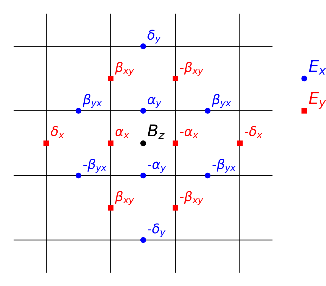This option allows the user to specify an extended stencil scheme that has been specifically optimised for the simulation grid spacing and timestep. See ⁵ for further details. or see 6 for stencil optimization code. Note that there is no option for changing the value of $\alpha_{x,y,z}$ since these are calculated using the following equations: $$ \begin{aligned} \alpha_x &= 1 - 2\beta_{xy} - 2\beta{xz} - 3\delta_x\,, \\\
\alpha_y &= 1 - 2\beta_{yx} - 2\beta{yz} - 3\delta_y\,, \\\
\alpha_z &= 1 - 2\beta_{zx} - 2\beta{zy} - 3\delta_z\,. \end{aligned} $$

• delta{x,y,z}, gamma{x,y,z}, beta{xy,xz,yx,yz,zx,zy} - The coefficients to use for the extended stencil points as shown in Figure [stencil]. See for further details. These coefficients are specified as floating point numbers. The default values are to set all coefficients to zero which results in $\alpha_{x,y,z}$ having values of unity. This corresponds to the standard Yee scheme.
• dt - The timestep restriction to use for the field solver

Strided Current Filtering

EPOCH 4.15 introduces strided multipass digital current filtering as described and benchmarked in the review by Vay and Godfrey. This can be tuned to substantially damp high frequencies in the currents and can be used to reduce the effect of numerical Cherenkov radiation. Once you turn on current filtering by specifying “smooth_currents=T” you can then set the following keys

• smooth_iterations - Integer number of iterations of the smoothing function to be performed. If not present defaults to one iteration. More iterations will produce smoother results but will be slower.
• smooth_compensation - Logical flag. If true then perform a compensation step (see Vay and Godfrey ⁶) after the smoothing steps are performed. Total number of iterations if true is smooth_iterations + 1. If not specified defaults to false
• smooth_strides - Either a comma separated list of integers or “auto” (without quote marks). This specifies the strides (in number of grid cells) to use when performing strided filtering. Specifying “1, 3” will smooth each point with the points immediately adjacent and with the points 3 cells away on each side of the current cell. Setting this key to “auto” uses a “1, 2, 3, 4” set of strides as a “good” starting point for strided filtering.

It should be stressed that there is no set of values that is guaranteed to give any given result from filtering while not affecting the physical correctness of your simulation. Current filtering should be tuned to match the problem that you want to work on and should always be carefully tested to ensure that it doesn’t produce unphysical results.

Dynamic Load Balancing

“dlb” in the input deck stands for Dynamic Load Balancing and, when turned on, it allows the code to rearrange the internal domain boundaries to try and balance the workload on each processor. This rearrangement is an expensive operation, so it is only performed when the maximum load imbalance reaches a given critical point. This critical point is given by the parameter “dlb_threshold” which is the ratio of the workload on the least loaded processor to the most loaded processor. When the calculated load imbalance is less than “dlb_threshold” the code performs a re-balancing sweep, so if “dlb_threshold = 1.0” is set then the code will keep trying to re-balance the workload at almost every timestep. At present the workload on each processor is simply calculated from the number of particles on each processor, but this will probably change in future. If the “dlb_threshold” parameter is not specified then the code will only be load balanced at initialisation time.

Automatic halting of a simulation

It is sometimes useful to be able to halt an EPOCH simulation midway through execution and generate a restart dump. Two methods have been implemented to enable this.

The first method is to check for the existence of a “STOP” file. Throughout execution, EPOCH will check for the existence of a file named either “STOP” or “STOP_NODUMP” in the simulation output directory. The check is performed at regular intervals and if such a file is found then the code exits immediately. If “STOP” is found then a restart dump is written before exiting. If “STOP_NODUMP” is found then no I/O is performed.

The interval between checks is controlled by the integer parameter “check_stop_frequency” which can be specified in the “control” block of the input deck. If it is less than or equal to zero then the check is never performed.

The next method for automatically halting the code is to stop execution after a given elapsed walltime. If a positive value for “stop_at_walltime” is specified in the control block of an input deck then the code will halt once this time is exceeded and write a restart dump. The parameter takes a real argument which is the time in seconds since the start of the simulation.

An alternative method of specifying this time is to write it into a separate text file. “stop_at_walltime_file” is the filename from which to read the value for “stop_at_walltime”. Since the walltime will often be found by querying the queueing system in a job script, it may be more convenient to pipe this value into a text file rather than modifying the input deck.

Requesting output dumps at run time

In addition to polling for the existence of a “STOP” file, EPOCH also periodically checks the output directory for a file named “DUMP”. If such a file is found then EPOCH will immediately create an output dump and remove the “DUMP” file. By default, the file written will be a restart dump but if the “DUMP” file contains the name of an output block then this will be used instead.

References

O. Buneman, “TRISTAN: The 3-D Electromagnetic Particle Code.” in Computer Space Plasma Physics: Simulations Techniques and Software, 1993. 1 ↩︎
S. Morris, D. O. Gericke, S. Fritzsche, J. Machado, J. P. Santos, and M. Afshari, “Recombination effects in laser-driven acceleration of heavy ions”, Phys. Rev. E 111, 065209, 2025 7 ↩︎
R. Lehe, A. Lifschitz, C. Thaury, V. Malka, and X. Davoine, “Numerical growth of emittance in simulations of laser-wakefield acceleration,” Phys. Rev. Accel. Beams, vol. 16, no. 2, p.021301, 2013 2. ↩︎
Pukhov, A., “Three-dimensional electromagnetic relativistic particle-in-cell code VLPL (Virtual Laser Plasma Lab)”, J. Plasma Phys., vol. 61, no. 3, p. 425, 1999 3. ↩︎
B. Cowan, D. Bruhwiler, J. Cary, E. Cormier-Michel, and C. Geddes, “Generalized algorithm for control of numerical dispersion in explicit time-domain electromagnetic simulations”, Phys. Rev. Accel. Beams, vol. 16, no. 4, p. 041303, 2013 4. ↩︎
A. Blinne, D. Schinkel, S. Kuschel, N. Elkina, S. G. Rykovanov, and M. Zepf, “A systematic approach to numerical dispersion in Maxwell solvers”, Computer Physics Communications, 00104655, 2017 5 ↩︎
J. L. Vay and B. B. Godfrey, “Modeling of relativistic plasmas with the particle-in-cell method”, Comptes Rendus Mcanique, 2014 6 ↩︎