Workshop examples
EPOCH workshop overview
The aims of the Workshop are:
- After the workshop you should be able to setup and run EPOCH on a problem of real importance to your research.
- You should also be in a position to use and understand the manual.
- You should learn about PIC codes in general.
- You should understand more about the pitfalls of trying to do LPI studies with PIC.
- Advice on how to run EPOCH and setup software on your home computers.
- Give advice to the EPOCH team on new features for the code.
Warwick EPOCH Personnel:
- Tony Arber – PI on EPOCH project at Warwick.
- Keith Bennett – PDRA and senior EPOCH developer.
- Chris Brady – Original EPOCH developer and head of RSE at Warwick
- Heather Ratcliffe - EPOCH user and developer
- Tom Goffrey – PDRA and developer on other non-EPOCH codes
- Alexander Seaton - Final year PhD student with extensive experience of using EPOCH
Resources:
- All machines, and exercises, are linux based.
- EPOCH is a Fortran90 program which uses MPI for parallelization.
- You will always need both F90 and MPI to compile and run the code even on one processor.
- MPI on a Windows computer is not easy. Use linux or a Mac.
Workstation usage
You can use the workstations for simple 1D tests and looking at the code.
Ultra-simple getting EPOCH guide!
These instructions should work in your host institute if you have git.
- Login to workstation using guest account.
- Open a terminal.
- Type the following command at the prompt:
git clone --recursive https://github.com/Warwick-Plasma/epoch.git
You will now have a directory called ‘epoch’. Inside this directory will be three EPOCH sub-directories epoch1d, epoch2d and epoch3d, an SDF directory and a few other files. Change directory into the epoch1d directory and start working through the ‘Getting Started with EPOCH’ guide.
Running the codes
Single core job: > echo Data | mpiexec -n 1 bin/epoch1d Four core
parallel job: > echo Data | mpiexec -n 4 bin/epoch2d
Note: If you don’t have git on your home computer you can always download a tar file of epoch when you return to your lab. This you get from the ‘Releases’ section on the EPOCH GitHub webpage. However I recommend you get, and learn, git and join the 21st century.
Getting Started with EPOCH
Compiling the code
The first thing you must do is to compile the code. This is done using the UNIX “make” command. This command reads a file called Makefile and uses the instructions in this file to generate all the steps required for compiling the code. Most of this is done automatically and the only part which typically needs changing are the instructions for which compiler to use and what compiler flags it accepts. The Makefiles supplied as part of the EPOCH source code contain sections for most commonly used compilers so it is usually unnecessary to actually edit these files. Usually you can compile just by passing the name of the compiler on the command line.
To compile the 1D version of the code, first change to the correct
directory by typing cd epoch/epoch1d. The compiler used on most
desktop machines is gfortran, so you can compile the code by typing
make COMPILER=gfortran. Alternatively, if you type
make COMPILER=gfortran -j4 then the code will be compiled in parallel
using 4 processors. If you wish, you can save yourself a bit of typing
by editing your ~/.bashrc file and adding the line
export COMPILER=gfortran at the top of the file. Then the command
would just be make -j4.
The most commonly used compiler on clusters these days is the Intel
FORTRAN compiler. You can compile by typing make COMPILER=intel or
edit your ~/.bashrc file to add the line export COMPILER=intel at the
top.
You should rarely need to edit the Makefile more than this. Occasionally, you may need to change fundamental behavior of the code by changing the list of flags in the “DEFINES” entry. This is documented in the User manual.
Running the code
Once you have built the version of EPOCH that you want (1D, 2D or 3D)
you simply run it by typing ./bin/epoch1d, ./bin/epoch2d, or
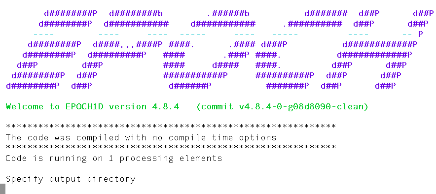
./bin/epoch3d. That will then show you the EPOCH splash page, which
prints the logo, lists any compile time options that you specified and
then asks you to specify the output directory. It will look in this
directory for a file with the name “input.deck” containing the problem
setup. Any output performed by the code will also be written into this
directory. To work through the examples, you must download an input deck
from the section below to the directory you want EPOCH to use and rename
the file “input.deck”. Throughout this guide we will assume that you use
the directory named “Data”.
Getting the example decks for this workshop
The example input decks used in this workshop can be downloaded using the following links. Create a directory “~/EXAMPLES” to put them in:
cd .
mkdir EXAMPLES
then download the .zip to this folder (either click the link and then copy the file, or right-click and select the save-as option). All decks as a .zip
01-1d_laser.deck - A simple laser
02-2d_laser.deck - A simple 2d laser
03-1d_two_stream.deck - A simple two-stream instability
04-1d_two_stream_io.deck - The same two-stream instability with extended output
05-2d_moving_window.deck - Simple moving-window problem with density jump and laser
06-2d_ramp.deck - Gaussian laser into a density ramp
07-1d_heating.deck - Demonstration of numerical heating
A Basic EM-Field Simulation
Our first example problem will be a simple 1D domain with a laser. This should give you a simple introduction to the input deck and visualization of 1D datasets.
Begin by copying the “01-1d_laser.deck” file from the EXAMPLES directory into the “Data” directory using the command: cp ~/EXAMPLES/01-1d_laser.deck Data/input.deck
Or click to expand and copy this text into a file "input.deck" in your Data directory.
begin:control
  nx = 200

  # Size of domain
  x_min = -4 * micron
  x_max = -x_min

  # Final time of simulation
  t_end = 50 * femto

  #stdout_frequency = 10
end:control


begin:boundaries
  bc_x_min = open
  #bc_x_min = simple_laser
  bc_x_max = open
end:boundaries


#begin:laser
#  boundary = x_min
#  intensity_w_cm2 = 1.0e15
#  lambda = 1 * micron
#  phase = pi / 2
#  t_profile = gauss(time, 2*micron/c, 1*micron/c)
#  t_end = 4 * micron / c
#end:laser
#
#
#begin:output
#  dt_snapshot = 1 * micron / c
#
#  # Properties on grid
#  grid = always
#  ey = always
#end:output
Open the input deck with an editor to view its contents. Eg. “gedit Data/input.deck”
This is the simplest possible input deck. The file is divided into blocks which are surrounded by “begin:blocktype” and “end:blocktype” lines. There are currently ten different blocktypes. The most basic input deck requires only two.
The first block is the “control” block. This is used for specifying the domain size and resolution and the length of time to run the simulation. There are also some global simulation parameters that can be specified in this block which will be introduced later. Within the block, each parameter is specified as a “name = value” pair.
The parameters are as follows. “nx” specifies the number of grid points in the x-direction (since this is a 1D code, the grid is only defined in the x-direction). “x_min” and “x_max” give the minimum and maximum grid locations measured in meters. Since most plasma simulations are measured in microns, there is a “micron” multiplication factor for convenience. There are also multiplication factors for “milli” through to “atto”. Finally, the simulation time is specified using “t_end” measured in seconds.
There are also commented lines in the deck. Any text following the “#” character is ignored. The character may appear anywhere on a line, so in the following example: t_end = 50 #* femto The value of “t_end” will be set to 50 seconds, since “#* femto” is ignored.
The other required block is the “boundaries” block. This contains one entry for each boundary, specifying what boundary condition to apply. For the 1D code there are two boundaries: “bc_x_min” and “bc_x_max”. The deck currently has both of these set to use open boundary conditions.
To run the code type: echo Data | mpiexec -n 4 ./bin/epoch1d
This will run epoch1d in parallel using 4 processors. It will use the directory named “Data” for all its output and will read the file “Data/input.deck” to obtain the simulation setup.
This simulation is rather dull. It is just a grid with zero electromagnetic field and it generates no data files. After running the program, two files are generated in the “Data” directory. The “deck.status” file contains the results from the deck parsing routines and is only useful for debugging. The “epoch1d.dat” file contains a terse one line header with the code name, version information and time the job started followed by a list of output dumps generated during the run.
Status information about the running job can be requested by uncommenting the “stdout_frequency” line in the “control” block. This is achieved by using a text editor to remove the “#” character and saving the file.
Adding a laser
We will now edit this input deck to add a laser source to the left hand boundary and dump some output files.
- Open the “Data/input.deck” file with an editor.
- Add a “#” comment character to the beginning of the first “bc_x_min” line in the “boundaries” block.
- Uncomment the line “bc_x_min = simple_laser”
- Uncomment the remaining lines in the file.
The change to the “boundaries” block instructs the code to add a laser source to the left-hand boundary.
The Laser Block
We then require a new block, named “laser”, to set up the laser source. The parameters in this block do the following:
- boundary – Specifies the boundary on which to attach this laser source
- intensity_w_cm2 – Specifies the intensity of the laser in Watts / cm^2
- lambda – Gives the wavelength of the laser in meters. We have used the multiplication factor “micron” for readability
- phase – Specifies the phase shift of the laser.
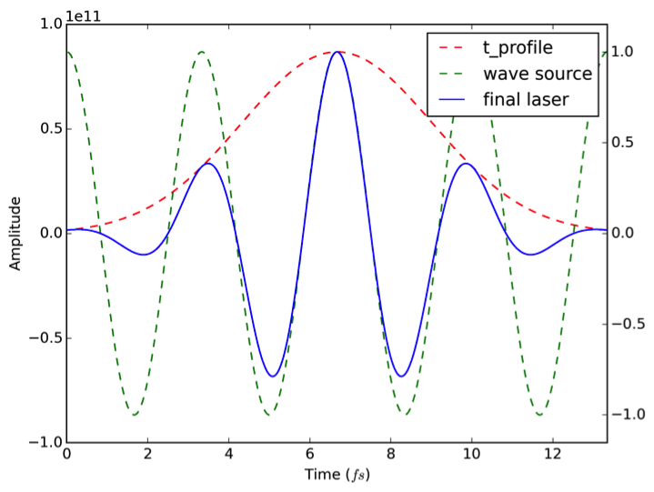
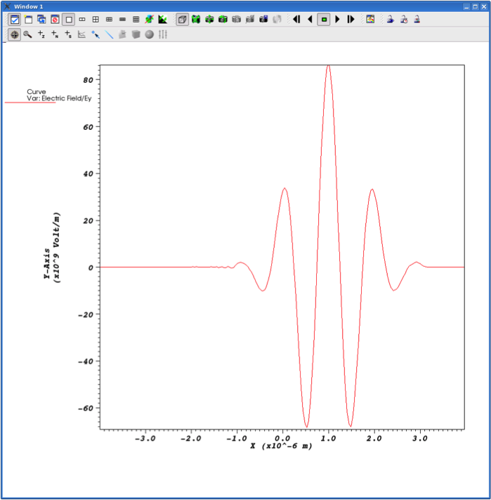
- t_profile – This parameter is used to modify the amplitude of the laser over time. It is usually used to ramp a laser up or down gradually. The left-hand side will be a function of time, usually ranging between zero and one.
- t_end – The time at which to switch off the laser.
These parameters are mostly self-explanatory. The “t_profile” parameter is best explained using an example. The figure above shows the result of using a gaussian time profile. The red line shows the value of “t_profile” over time. This starts at a value close to zero, ramps up to one and then ramps back down to zero. The green line shows the amplitude of the laser when “t_profile” has not been specified. Note that the function would normally be a sine wave, but this has been shifted by pi/2 because the “phase” parameter was used. The blue line shows the laser amplitude generated when the “t_profile” gaussian profile is applied.
The Output Block
The final addition is the “output” block. We will cover this in more detail later. For now, it is sufficient to know that this is the block which controls the generation of data output. The parameters used in this case are:
- dt_snapshot – This specifies the simulation time between each output dump
- grid – This controls when to dump the simulation grid. The value of “always” means that the grid will be output whenever there is a new output dump generated.
- ey – The controls when to dump the y-component of the electric field.
Visualising the data
Now that we have generated some data we need to plot it. The data is written to a self-describing file format called SDF. This has been developed for use by several codes maintained at the University of Warwick. There are routines for reading the data from within IDL, VisIt, MatLab and Python.
More complete documentation on visualisation routines is available here
Loading the data into IDL/GDL
First, we will load the data into IDL/GDL. The desktop machines have GDL
installed – the GNU Data Language, which is a free implementation of
IDL. It doesn’t have all the feature of IDL but the core routines and
syntax are identical. Type gdl Start.pro and GDL will start up and
load the SDF reading library. To view the data contained in a file, type
list_variables,7,'Data' Here, “7” is the snapshot number. It can be
any number between 0 and 9999. The second parameter specifies the
directory which holds the data files. If it is omitted then the
directory named “Data” is used by default.
To load the data and assign the result to a structure named “data”, just
issue the following command: data = getstruct(7,/varname) Here,
“/varname” is any of the variables listed by the previous command. This
will just read the “varname” variable into the data structure. However,
it is usually easiest just to omit the “/varname” flag. If it is omitted
then the entire contents of the file is read.
The “getstruct” command returns a hierarchical data structure. The
contents of this structure can be viewed with the following command:
help,data,/struct For the current example the result of this command
is the following:
 GDL> help,data,/struct
** Structure <Anonymous>, 8 tags, data length=5552:
   FILENAME        STRING    'Data/0007.sdf'
   TIMESTEP        LONG               185
   TIME            DOUBLE       2.3449556e-14
   HEADER          STRUCT    -> <Anonymous> Array[1]
   ELAPSED_TIME    STRUCT    -> <Anonymous> Array[1]
   EY              STRUCT    -> <Anonymous> Array[1]
   GRID            STRUCT    -> <Anonymous> Array[1]
   X               DOUBLE    Array[200]
The first few entries are fairly self-explanatory. The seventh item is a 1D array containing the cell-centred grid positions. The fiftth item is a structure containing a 1D array of Ey at these positions. This structure can be queried in the same way as “data” :
 GDL> help,data.ey,/struct
** Structure <Anonymous>, 2 tags, data length=1728:
   METADATA        STRUCT    -> <Anonymous> Array[1]
   DATA            DOUBLE    Array[200]
The raw data is contained in the “data” entry. The sixth entry, “GRID” is a structure which contains :
GDL> help,data.grid,/struct
** Structure <Anonymous>, 5 tags, data length=1824:
   METADATA        STRUCT    -> <Anonymous> Array[1]
   X               DOUBLE    Array[201]
   LABELS          STRING    Array[1]
   UNITS           STRING    Array[1]
   NPTS            LONG      Array[1]
This is the node-centred grid along with its metadata. The cell-centred array shown previously is derived from this. Finally, the HEADER entry contains metadata about the code and runtime information.
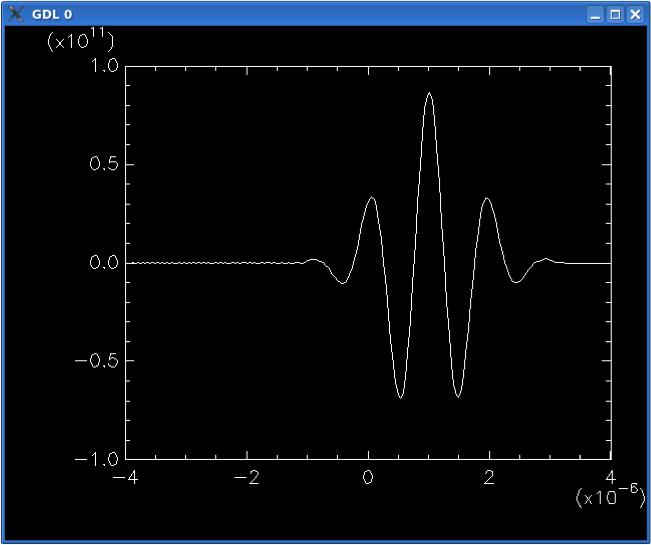
The above plot can be generated by issuing the following command:
plot,data.x,data.ey.data There are more examples on using idl/gdl in
the
manual.
Loading the data into Python
EPOCH also ships with a module for reading SDF data into python. To build this module, change directory to epoch/epoch1d (or 2d,3d) and type “make sdfutils”. This will build the python reader and install it locally. It also installs a helper module which adds a few user-friendly routines. To simplify discussion, we will just focus on using this helper routine.
Open a python interpreter by typing “python”, or preferably “ipython” if you have it installed.
On the desktops, the sdf and sdf_helper modules will be imported for you, as sdf and sdf_helper respectively. On other machines, to load the SDF module, type the command:
import sdf_helper as sh
You can now load a data file by typing:
data = sh.getdata(7)
or
data = sdf_helper.getdata(7)
This returns a data structure which can be inspected using
data.__dict__
It also imports the contents of data arrays and prints a summary of what has been imported.
For example:
from sdf_helper import *
data = getdata(7)
#>>Reading file Data/0007.sdf
t() = time
ey(200,) = ey
x(201,) = grid
xc(200,) = grid_mid
If you have matplotlib installed then you can load the module using
from matplotlib.pyplot import *
Turn on interactive plotting with
ion()
You can now plot the data with the command:
plot(xc,ey)
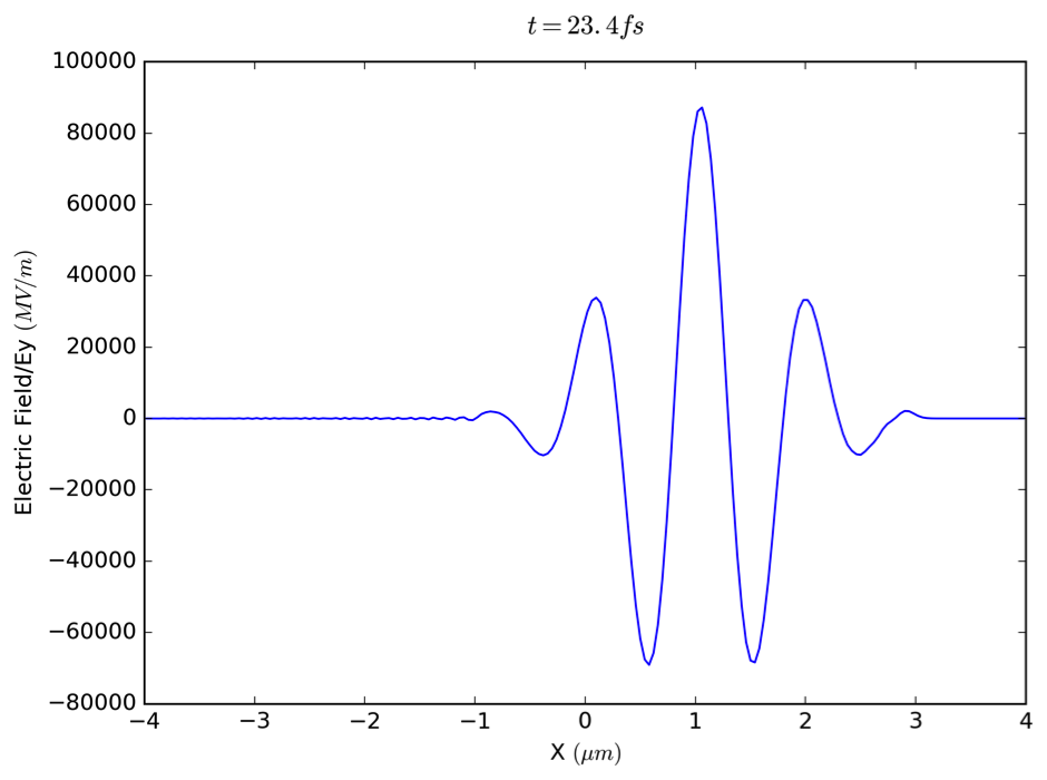
The helper module has a “plot_auto” command which automatically adds axis labels. To use this type:
plot_auto(data.Electric_Field_Ey)
Loading the data into VisIt
EPOCH comes with an SDF reader plugin for the VisIt parallel visualization tool. In order to use it, you must first compile the reader to match the version of VisIt installed on your system. To do this, first ensure that the “visit” command is in your path. This is the case if typing “visit” on the command line launches the VisIt application. Once you have this setup, you should be able to type “make visit” from one of the epoch{1,2,3}d directories. You will need to re-do this each time a new version of VisIt is installed on your system.
Launch the VisIt application by typing “visit” on the command line. A
useful shortcut is to type visit -o Data/0000.sdf. This will launch
VisIt and open the specified data file on startup. Alternatively, you
can browse for the file to open using the “Open” button. All the SDF
files in a directory will be grouped together with a green “DB” icon and
the name “*.sdf database”.
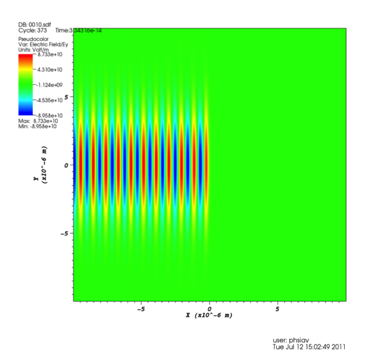
You can then plot a quantity by pressing the “Add” button, selecting the type of plot and the variable to use for the plot. When the plot has been selected, press the “Draw” button to render it to screen. The plot above was generated by selecting “Add->Curve->Electric Field->Ey”. Some of the plot properties were adjusted to make it look nicer.
More details on using VisIt are here. We recommend that you learn VisIt – it’s free and powerful.
Loading data into MatLab
The EPOCH distribution also comes with a set of reader routines for the MatLab plotting utility. The routines themselves are contained in the “Epoch/Matlab” directory. It is first necessary to add this directory to your search path. One simple way of doing this is to use the menu item “File->Set Path” and then “Add Folder” to select the location of the “Matlab” folder. To make this change permanent you have to use the “Save” button. Unfortunately, on many systems this will not work as it tries to change global settings which will not be permitted on a multi-user setup. On Unix systems (including OS X), the change can be made permanent by using the “$MATLABPATH” environment variable. For example in bash this would be ‘export MATLABPATH=“Epoch/Matlab” ' which you can add to your .bashrc file.
To load the data from an SDF file, type the following at the MatLab prompt:
data=GetDataSDF('Data/0007.sdf');
The “data” variable will now contain a data structure similar to that obtained with the IDL reader. You can explore the contents of the structure using MatLab’s built-in variable editor. To plot Ey, you can browse to “data.Electric_Field.Ey”. The structure member “data.Electric_Field.Ey.data” contains the 1D array with Ey values. Right-clicking on it gives a range of options, including “plot”. Alternatively, from the command prompt you can type
 x=data.Electric_Field.Ey.grid.x;
 xc=(x(1:end-1) + x(2:end))/2;
 plot(xc,data.Electric_Field.Ey.data);
The first two lines set up a cell-centred grid using the node-centred grid data. In the future, this work will be automatically done by the reader.
A 2D laser
Next, we will take a look at the 2-dimensional version of the code.
- Change to the epoch2d directory:
cd ~/Epoch/epoch2d - Type
make -j4to compile the code. - Copy the next example input deck into the Data directory:
cp ~/EXAMPLES/02-2d_laser.deck Data/input.deckor save the text below into Data/input.deck - Run with
echo Data | mpirun -np 4 ./bin/epoch2d
Click to expand
begin:control
  nx = 500
  ny = nx

  # Size of domain
  x_min = -10 * micron
  x_max = -x_min
  y_min = x_min
  y_max = x_max

  # Final time of simulation
  t_end = 50 * femto

  stdout_frequency = 10
end:control


begin:boundaries
  bc_x_min = simple_laser
  bc_x_max = open
  bc_y_min = periodic
  bc_y_max = periodic
end:boundaries


begin:constant
  lambda0 = 1 * micron
  theta = pi / 8.0
end:constant


begin:laser
  boundary = x_min
  intensity_w_cm2 = 1.0e15
  lambda = lambda0 * cos(theta)
  profile = gauss(y, 0, 4*micron)
  #phase = -2.0 * pi * y * tan(theta) / lambda0
  #t_profile = gauss(time, 2*micron/c, 1*micron/c)
end:laser


begin:output
  dt_snapshot = 1 * micron / c

  # Properties on grid
  grid = always
  ex = always
  ey = always
  ez = always
  bx = always
  by = always
  bz = always
end:output
This deck is very similar to the 1D version that we have just looked at. It contains the necessary modifications for adding a new dimension and some additions to the laser block for driving a laser at an angle.
The “control” block now contains “ny” which specifies the number of grid points in the y-direction. Notice that we are using the value “nx” to set “ny”. As soon as “nx” has been assigned it becomes available as a constant for use as part of a value. We must also provide the minimum and maximum grid positions in the y-direction using “y_min”, “y_max”. Like “nx”, the values “x_min” and “x_max” are available for use once they have been assigned.
In the “boundaries” block we must include boundary conditions for the lower and upper boundaries in the y-direction, “bc_y_min”, “bc_y_max”. These have both been set to “periodic” so that the field at the top of the domain wraps around to the bottom of the domain.
Next, we introduce a new block type, “constant”. This block defines named variables which can be arbitrary mathematical expressions. Once defined, these can be used on the left-hand side of name-value pairs in the same way we used “nx”, “x_min”, etc. in the “control” block. This facility can greatly aid the construction and maintenance of complex input decks.
The “laser” block is similar to that given in the 1D version except that there is now a “profile” parameter. In a similar manner to “t_profile” this is a function ranging between 0 and 1 which is multiplied by the wave amplitude to give a modified laser profile. The only difference is that this is a function of space rather than time. When applied to a laser attached to “x_min” or “x_max” it is a function of Y, defined at all points along the boundary. When the laser is attached to “y_min” or “y_max”, it is a function of X.
Finally, the output block has been modified so that it outputs all electromagnetic field components.
The result of plotting “Add->Pseudocolor->Electric Field->Ey” in
VisIt is shown above. 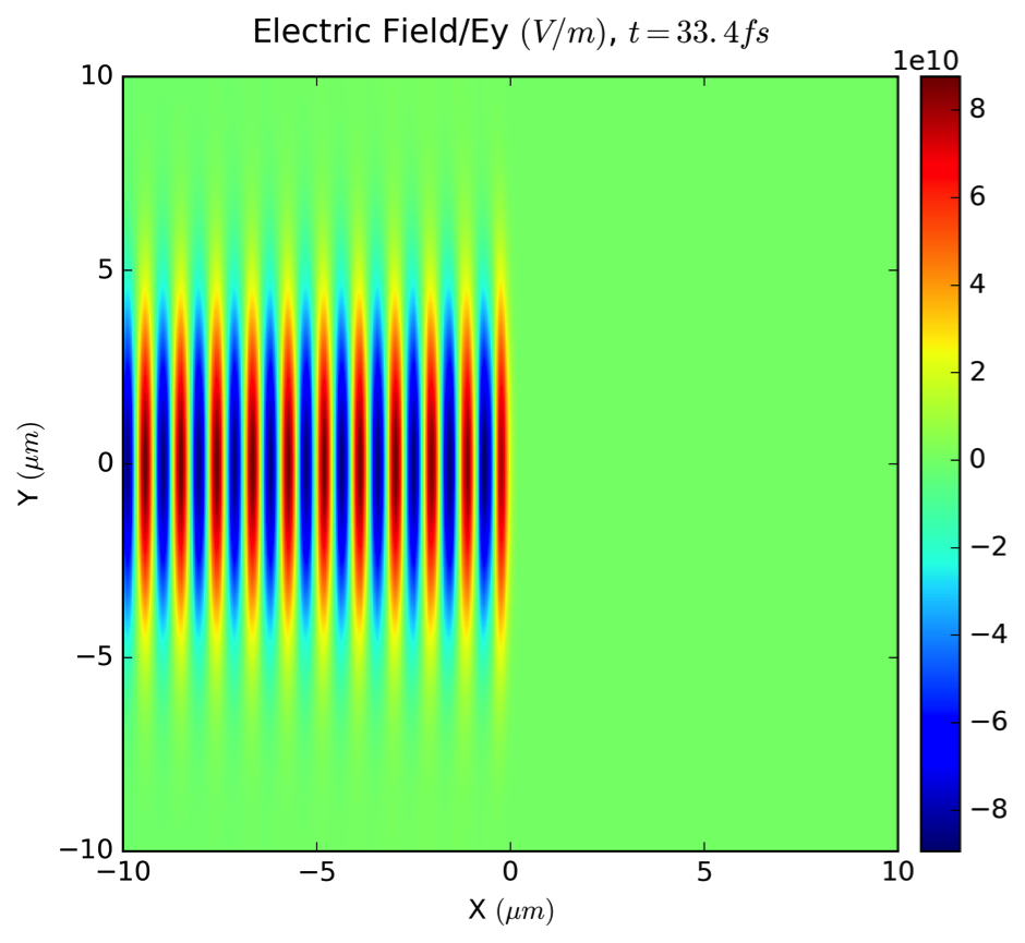
The laser block also contains a commented-out “phase” entry. Unlike in the 1D version seen previously, this is a function of Y, like the “profile” parameter. Uncommenting this line and re-running the deck will generate a laser driven at an angle to the boundary. The mathematical details explaining why this works are explained in more detail in the User Manual. By making the value of “theta” a function of Y, it is also possible to produce a focused laser. This is left as an exercise for the reader!
The above plot can also be generated using matplotlib using the command
plot2d(data.Electric_Field_Ey)
Specifying particle species
In this example we will finally introduce some particles into the PIC code! The deck is for the 1D version of the code, so change back to the epoch1d directory and copy ~/EXAMPLES/03-1d_two_stream.deck to Data/input.deck (or copy the deck below) and run the code.
Click to expand
begin:control
  nx = 400

  # Size of domain
  x_min = 0
  x_max = 5.0e5

  # Final time of simulation
  t_end = 1.5e-1

  stdout_frequency = 400
end:control


begin:boundaries
  bc_x_min = periodic
  bc_x_max = periodic
end:boundaries


begin:constant
  drift_p = 2.5e-24
  temp = 273
  dens = 10
end:constant


begin:species
  # Rightwards travelling electrons
  name = Right
  charge = -1
  mass = 1.0
  temp = temp
  drift_x = drift_p
  number_density = dens
  npart = 4 * nx
end:species


begin:species
  # Leftwards travelling electrons
  name = Left
  charge = -1
  mass = 1.0
  temp = temp
  drift_x = -drift_p
  number_density = dens
  npart = 4 * nx
end:species


begin:output
  # Number of timesteps between output dumps
  dt_snapshot = 1.5e-3

  # Properties at particle positions
  particles = always
  px = always

  # Properties on grid
  grid = always
  ey = always
end:output
The control block has one new parameter. “npart” gives the total number of PIC particles to use in the simulation.
The input deck contains a new block type, “species”, which is used for populating the domain with particles. Every species block must contain a “name” parameter. This is used to identify the particle species in other sections of the input deck and is also used for naming variables in the output dumps. The next parameter is “charge” which gives the charge on each particle in terms of elementary charge units. “mass” is specified in units of electron mass. “frac” is the fraction of the total number of PIC particles (npart) to assign to this species. Both of the blocks in this deck use “frac = 0.5”, so there will be 1600 particles of each species. The next parameter, “temp”, sets the average temperature of the particle species in Kelvin. Alternatively, you can use “temp_ev” to specify the temperature in electronvolts. Particles are assigned an initial momentum corresponding to a Maxwell-Boltzmann distribution for this temperature. It is defined across the entire problem domain, so in 1D it is a function of X, in 2D a function of X and Y, and in 3D a function of X, Y and Z. “number_density” sets the number density across the problem domain. The code is set to use per-particle weights in the default Makefile. With this option, the pseudoparticles are distributed evenly across the domain. Then the weight of each pseudoparticle is adjusted so that it matches the number density specified in the “number_density” parameter. The alternative option is to disable per-particle weighting. In this case, the weight of each pseudoparticle is the same and the particles are placed on the grid so that they match the number density at the start of the simulation. Finally, we have a “drift_x” parameter. This is also defined across the entire problem domain and is used to give the particles an average momentum drift in the x-direction. There are similar “drift_y” and “drift_z” parameters.
This deck has been designed to simulate a two-stream instability, so it
has two groups of particles which are identical in every respect except
that one set is drifting in the opposite direction to the other. 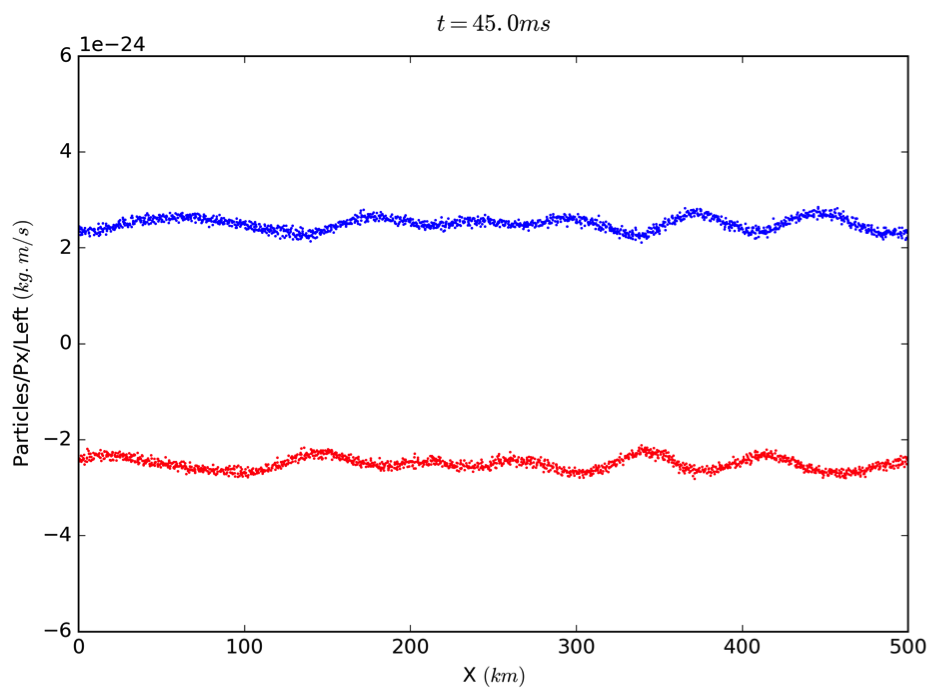
In the output block we have added a couple of parameters for outputting particle data. The first parameter, “particles”, outputs the grid on which the particles are defined. There are two different types of variable in EPOCH: particle variables and grid-based variables. The grid-based variables are like the electromagnetic field components we have seen previously. The domain is divided into a regular Cartesian mesh and the grid-based variables are defined at either a node or cell-centre of each point in this mesh. Particle variables, on the other hand, are associated with each of the pseudoparticles. These PIC particles move independently of the Cartesian mesh and can be located anywhere in the problem domain. The “particles” parameter requests that the coordinates of each particle are written to file. This information is required in order to plot any of the particle variables. The next parameter is “px” which writes the momentum of each particle.
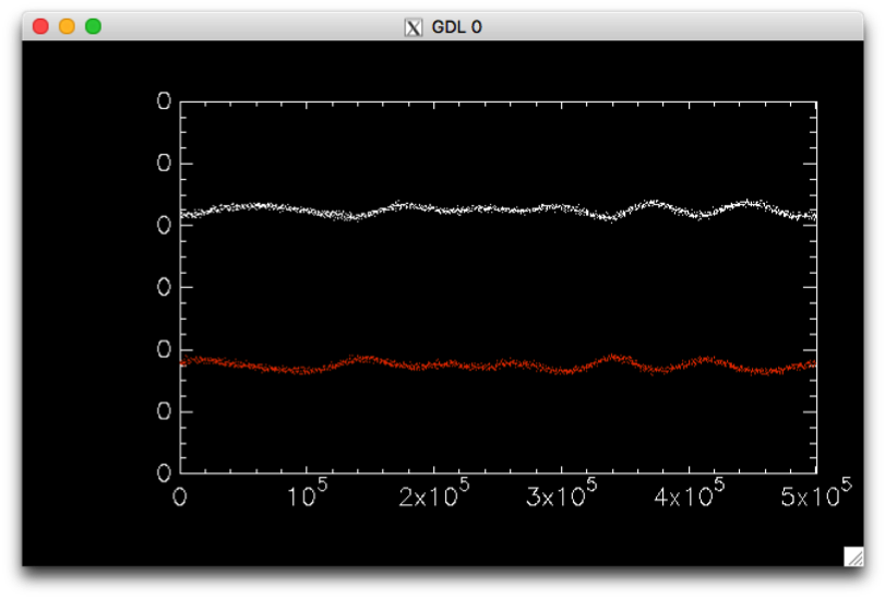
To plot this using python and matplotlib, type the following:
data = getdata(30)
plot1d(data.Particles_Px_Left,'r.',ms=2,yscale=1)
oplot1d(data.Particles_Px_Right,'b.',ms=2,yscale=1)
ylim([-6e-24,6e-24])
To plot with GDL, type the following:
gdl Start.pro

data=getstruct(30)
plot,data.grid_right.x,data.px_right.data,psym=3,$
  yrange=[-6e-24,6e-24],ystyle=1
oplot,data.grid_left.x,data.px_left.data,psym=3,color=150
Above we have plotted the x-component of particle momentum as a function of x-position at a time when the instability is just starting to form. The “psym=3” option to the plot routine tells GDL to plot each data point as a dot and not to join the dots up.
The Output Block
The contents of the output block can be much more complicated than the examples shown so far. Here, we will cover the options in a little more depth.
EPOCH currently has three different types of output dump. So far, we have only been using the “normal” dump type. The next type of dump is the “full” dump. To request this type of dump, you add the parameter “full_dump_every” which is set to an integer. If this was set equal to “10” then after every 9 dump files written, the 10th dump would be a “full” dump. This hierarchy exists so that some variables can be written at frequent intervals whilst large variables such as particle data are written only occasionally. The third dump type is the “restart” dump. This contains all the variables required in order to restart a simulation, which includes all the field variables along with particle positions, weights and momentum components. In a similar manner to full dumps, the output frequency is specified using the “restart_dump_every” parameter.
So far, we have given all the variable parameters a value of “always” so that they will always be dumped to file. There are three other values which can be used to specify when a dump will occur. “never” indicates that a variable should never be dumped to file. This is the default used for all output variables which are not specified in the output block. The value of “full” indicates that a variable should be written at full dumps. “restart” means it is written into restart dumps.
There are a few output variables which are grid-based quantities derived by summing over properties for all the particles contained within each cell on the mesh. These are “ekbar”, “mass_density”, “charge_density”, “number_density” and “temperature”. To find more details about these variables, consult the output block section of the user manual.