In this section we outline a few worked examples of setting up problems using the EPOCH input deck.

Electron two stream instability

An obvious simple test problem to do with EPOCH is the electron two stream instability. An example of a nice dramatic two stream instability can be obtained using EPOCH1D by setting the code with the following input deck file:

begin:control
   nx = 400

   # Size of domain
   x_min = 0
   x_max = 5.0e5

   # Final time of simulation
   t_end = 1.5e-1

   stdout_frequency = 400
end:control


begin:boundaries
   bc_x_min = periodic
   bc_x_max = periodic
end:boundaries


begin:constant
   drift_p = 2.5e-24
   temp = 273
   dens = 10
end:constant


begin:species
   # Rightwards travelling electrons
   name = Right
   charge = -1
   mass = 1.0
   temp = temp
   drift_x = drift_p
   number_density = dens
   npart = 4 * nx
end:species


begin:species
   # Leftwards travelling electrons
   name = Left
   charge = -1
   mass = 1.0
   temp = temp
   drift_x = -drift_p
   number_density = dens
   npart = 4 * nx
end:species


begin:output
   # Number of timesteps between output dumps
   dt_snapshot = 1.5e-3

   # Properties at particle positions
   particles = always
   px = always

   # Properties on grid
   grid = always
   ex = always
   ey = always
   ez = always
   bx = always
   by = always
   bz = always
   jx = always
   ekbar = always
   mass_density = never + species
   charge_density = always
   number_density = always + species
   temperature = always + species
end:output

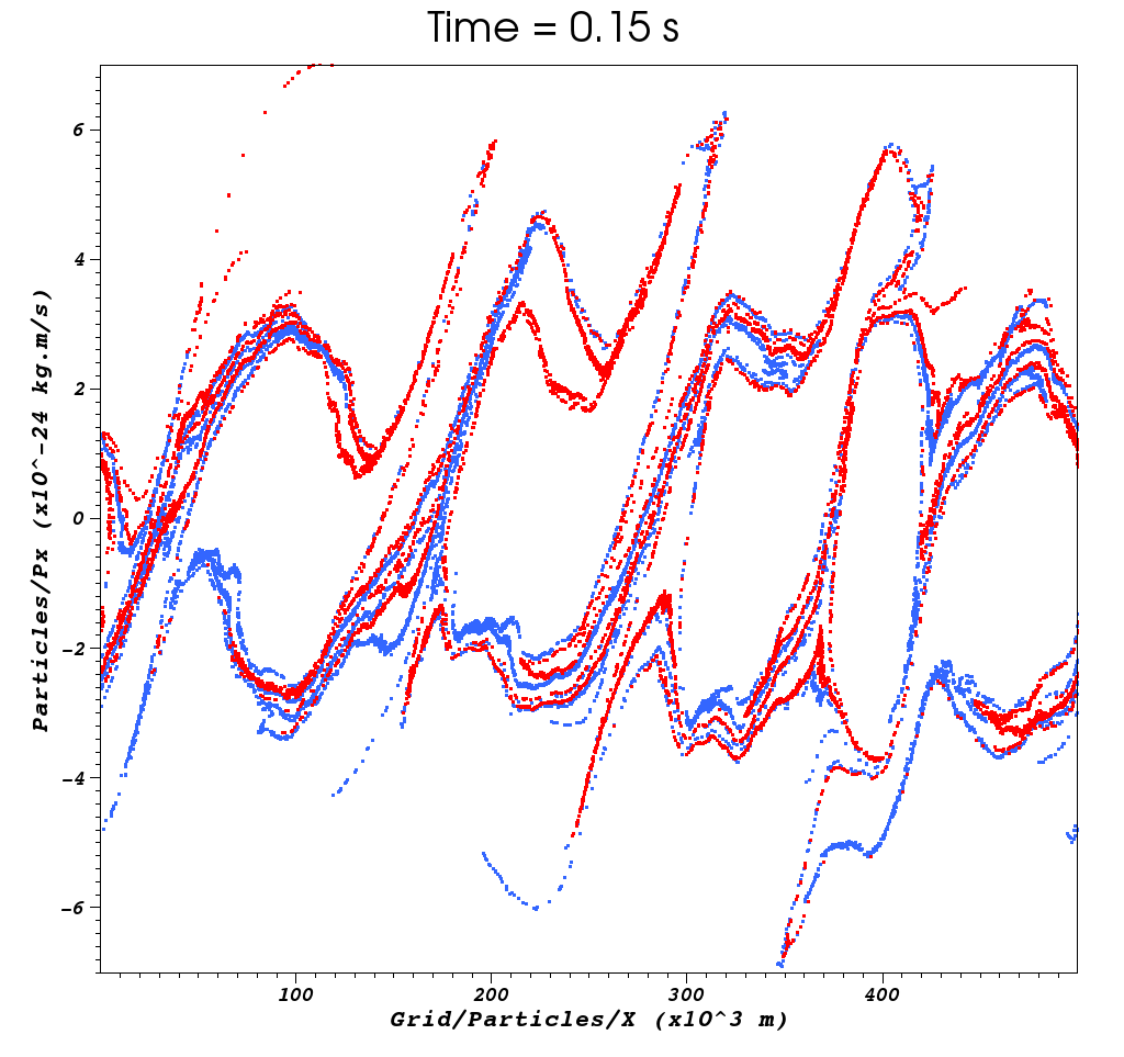In this example, the constant block sets up constants for the momentum space drift, the temperature and the electron number density. The two species blocks set up the two drifting Maxwellian distributions and the constant density profile. The final output from this simulation is shown in the figure.

Structured density profile in EPOCH2D

A simple but useful example for EPOCH2D is to have a highly structured initial condition to show that this is still easy to implement in EPOCH. A good example initial condition would be:

begin:control
   nx = 500
   ny = nx
   x_min = -10 * micron
   x_max = -x_min
   y_min =  x_min
   y_max =  x_max
   nsteps = 0
end:control

begin:boundaries
   bc_x_min = periodic
   bc_x_max = periodic
   bc_y_min = periodic
   bc_y_max = periodic
end:boundaries

begin:constant
   den_peak = 1.0e19
end:constant

begin:species
   name = Electron
   number_density = den_peak * (sin(4.0 * pi * x / length_x + pi / 4)) \
                    * (sin(8.0 * pi * y / length_y) + 1)
   number_density_min = 0.1 * den_peak
   charge = -1.0
   mass = 1.0
   npart = 20 * nx * ny
end:species

begin:species
   name = Proton
   number_density = number_density(Electron)
   charge = 1.0
   mass = 1836.2
   npart = 20 * nx * ny
end:species

begin:output
   number_density = always + species
end:output

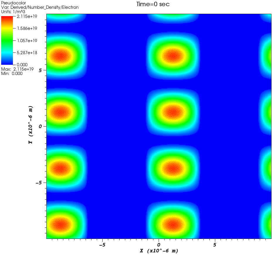
The species block for Electron is specified first, setting up the electron density to be a structured 2D sinusoidal profile. The species block for Proton is then set to match the density of Electron, enforcing charge neutrality. On its own this initial condition does nothing and so only needs to run for 0 timesteps (nsteps = 0 in input.deck). The resulting electron number density should look like the figure.

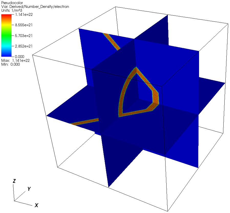
A hollow cone in 3D

A more useful example of an initial condition is to create a hollow cone. This is easy to do in both 2D and 3D, but is presented here in 3D form.

begin:control
   nx = 250
   ny = nx
   nz = nx
   x_min = -10 * micron
   x_max = -x_min
   y_min = x_min
   y_max = x_max
   z_min = x_min
   z_max = x_max
   nsteps = 0
end:control

begin:boundaries
   bc_x_min = simple_laser
   bc_x_max = simple_outflow
   bc_y_min = periodic
   bc_y_max = periodic
   bc_z_min = periodic
   bc_z_max = periodic
end:boundaries

begin:output
   number_density = always + species
end:output

begin:constant
   den_cone = 1.0e22
   ri = abs(x - 5.0e-6) - 0.5e-6
   ro = abs(x - 5.0e-6) + 0.5e-6
   xi = 3.0e-6 - 0.5e-6
   xo = 3.0e-6 + 0.5e-6
   r = sqrt(y^2 + z^2)
end:constant

begin:species
   name = proton
   charge = 1.0
   mass = 1836.2
   number_density = if((r gt ri) and (r lt ro), den_cone, 0.0)
   number_density = if((x gt xi) and (x lt xo) and (r lt ri), \
                       den_cone, number_density(proton))
   number_density = if(x gt xo, 0.0, number_density(proton))
   npart = nx * ny * nz
end:species

begin:species
   name = electron
   charge = -1.0
   mass = 1.0
   number_density = number_density(proton)
   npart = nx * ny * nz
end:species

Cone initial conditions in 3D

Cone initial conditions in 2D

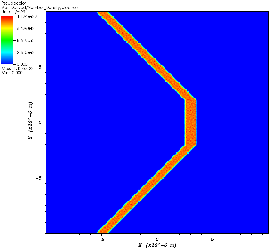
To convert this to 2D, simply replace the line r = sqrt(y^2+z^2) with the line r = abs(y). The actual work in these initial conditions is done by the three lines inside the block for the Proton species. Each of these lines performs a very specific function:

1. Creates the outer cone. Simply tests whether r is within the range of radii which corresponds to the thickness of the cone and if so fills it with the given density. Since the inner radius is x dependent this produces a cone rather than a cylinder. On its own, this line produces a pair of cones joined at the tip.
2. Creates the solid tip of the cone. This line just tests whether the point in space is within the outer radius of the cone and within a given range in x, and fills it with the given density if true.
3. Cuts off all of the cone beyond the solid tip. Simply tests if x is greater than the end of the cone tip and sets the density to zero if so.

This deck produces an initial condition as in the Figures in 3D and 2D respectively.