Using EPOCH in practice
Specifying initial conditions for particles using the input deck
If the initial conditions for the plasma you wish to model can be described by a number density and temperature profile on the underlying grid then EPOCH can create an appropriate particle distribution for you. The set of routines which accomplish this task are known as the autoloader. For many users, this functionality is sufficient to make use of the code and there is no need to deal with the internal representation of particles in EPOCH.
The autoloader randomly loads particles in space to reproduce the number density profile that was requested. It then sets the momentum components of the particles to approximate a Maxwell-Boltzmann distribution corresponding to the temperature profile. Sometimes this is not the desired behaviour, for example you may wish to model a bump-on-tail velocity distribution. It is currently not possible to specify these initial conditions from the input deck and the particles must be setup by modifying the source code.
There are two stages to the particle setup in EPOCH
- auto_load - This routine is called after reading and parsing the input deck. It takes care of allocating particles and setting up their initial positions and momenta using the initial conditions supplied in deck file. It is not necessary to recompile the code, or even have access to the source to change the initial conditions using this method.
- manual_load - Once particles have been allocated they can have their properties altered in this routine. By default it is an empty routine which does nothing.
Setting autoloader properties from the input deck
To illustrate using the autoloader in practice, we present an example for setting up an isolated plasma block in 2D. This would look like:
begin:species
   name = s1
   # First set number_density in the range 0 > 1
   # Cut down number_density in x direction
   number_density = if ((x gt -1) and (x lt 1), 1.0, 0.2)
   # Cut down number_density in y direction
   number_density = if ((y gt -1) and (y lt 1), number_density(s1), 0.2)

   # Multiply number_density by real particle number_density
   number_density = number_density(s1) * 100.0

   # Set the temperature to be zero
   temp_x = 0.0
   temp_y = temp_x(s1)

   # Set the minimum number_density for this species
   number_density_min = 0.3 * 100.0
end:species

begin:species
   # Just copy the number_density for species s1
   number_density = number_density(s1)

   # Just copy the temperature from species s1
   temp_x = temp_x(s1)
   temp_y = temp_y(s1)

   # Set the minimum number_density for this species
   number_density_min = 0.3 * 100.0
end:species
An important point to notice is that the two parts of the logical expressions in the input deck are enclosed within their own brackets. This helps to remove some ambiguities in the functioning of the input deck parser. It is hoped that this will soon be fixed, but at present ALWAYS enclose logical expressions in brackets.
Manually overriding particle parameters set by the autoloader
Since not all problems in plasma physics can be described in terms of an
initial distribution of thermal plasma, it is also possible to manually
control properties of each individual pseudoparticle for an initial
condition. This takes place in the subroutine manual_load in the file
user_interaction/ic_module.f90. Manual loading takes place after all
the autoloader phase, to allow manual tweaking of autoloader specified
initial conditions.
EPOCH internal representation of particles
Before we can go about manipulating particle properties in
manual_load, we first need an overview of how the particles are
defined in EPOCH. Inside the code, particles are represented by a
Fortran90 TYPE called particle. The current definition of this
type (in 1D) is:
  TYPE particle
    REAL(num), DIMENSION(3) :: part_p
    REAL(num) :: part_pos
#if !defined(PER_SPECIES_WEIGHT) || defined(PHOTONS)
    REAL(num) :: weight
#endif
#ifdef DELTAF_METHOD
    REAL(num) :: pvol
#endif
#ifdef PER_PARTICLE_CHARGE_MASS
    REAL(num) :: charge
    REAL(num) :: mass
#endif
    TYPE(particle), POINTER :: next, prev
#ifdef PARTICLE_DEBUG
    INTEGER :: processor
    INTEGER :: processor_at_t0
#endif
#ifdef PARTICLE_ID4
    INTEGER :: id
#elif PARTICLE_ID
    INTEGER(i8) :: id
#endif
#ifdef WORK_DONE_INTEGRATED
    REAL(num) :: work_x
    REAL(num) :: work_y
    REAL(num) :: work_z
    REAL(num) :: work_x_total
    REAL(num) :: work_y_total
    REAL(num) :: work_z_total
#endif
#ifdef PHOTONS
    REAL(num) :: optical_depth
    REAL(num) :: particle_energy
#ifdef TRIDENT_PHOTONS
    REAL(num) :: optical_depth_tri
#endif
#endif
  END TYPE particle
Here, most of the preprocessing directives have been stripped out for
clarity. We have left #ifdef PARTICLE_DEBUG as an example. Here, the
“processor” and “processor_at_t0” variables only exist if the
-DPARTICLE_DEBUG define was put in the makefile. If you want to access
a property that does not seem to be present, check the
preprocessor
defines.
The “particle” properties can be explained as follows:
- part_p - The momentum in 3 dimensions for the particle. This is always of size 3.
- part_pos - The position of the particle in space. This is of the same size as the dimensionality of the code.
- weight - The weight of this particle. The number of real particles represented by this pseudoparticle.
- charge - The particle charge. If the code was compiled without per particle charge, then the code uses the charge property from TYPE(particle_species).
- mass - The particle rest mass. If the code was compiled without per particle mass, then the code uses the mass property from TYPE(particle_species).
- next, prev - The next and previous particle in the linked list which represents the particles in the current species. This will be explained in more detail later.
- processor - The rank of the processor which currently holds the particle.
- processor_at_t0 - The rank of the processor on which the particle started.
- id - Unique particle ID.
- optical_depth - Optical depth used in the QED routines.
- particle_energy - Particle energy used in the QED routines.
- optical_depth_tri - Optical depth for the trident process in the QED routines.
Collections of particles are represented by another Fortran TYPE, called
particle_list. This type represents all the properties of a
collection of particles and is used behind the scenes to deal with
inter-processor communication of particles. The definition of the type
is:
  TYPE particle_list
    TYPE(particle), POINTER :: head
    TYPE(particle), POINTER :: tail
    INTEGER(i8) :: count
    INTEGER :: id_update
    ! Pointer is safe if the particles in it are all unambiguously linked
    LOGICAL :: safe

    ! Does this partlist hold copies of particles rather than originals
    LOGICAL :: holds_copies

    TYPE(particle_list), POINTER :: next, prev
  END TYPE particle_list
- head - The first particle in the linked list.
- tail - The last particle in the linked list.
- count - The number of particles in the list. Note that this is NOT MPI aware, so reading count only gives you the number of particles on the local processor.
- safe - Any particle_list which a user should come across will be a safe particle_list. Don’t change this property.
- next, prev - For future expansion it is possible to attach particle_lists together in another linked list. This is not currently used anywhere in the code.
An entire species of particles is represented by another Fortran TYPE,
this time called particle_species. This represents all the
properties which are common to all particles in a species. The current
definition is:
  TYPE particle_species
    ! Core properties
    CHARACTER(string_length) :: name
    TYPE(particle_species), POINTER :: next, prev
    INTEGER :: id
    INTEGER :: dumpmask
    INTEGER :: count_update_step

    REAL(num) :: charge
    REAL(num) :: mass
    REAL(num) :: weight
    INTEGER(i8) :: count
    TYPE(particle_list) :: attached_list
    LOGICAL :: immobile
    LOGICAL :: fill_ghosts

    ! Parameters for relativistic and arbitrary particle loader
    INTEGER :: ic_df_type
    REAL(num) :: fractional_tail_cutoff

    TYPE(primitive_stack) :: dist_fn
    TYPE(primitive_stack) :: dist_fn_range(3)

#ifndef NO_TRACER_PARTICLES
    LOGICAL :: zero_current
#endif

    ! ID code which identifies if a species is of a special type
    INTEGER :: species_type

    ! particle cell division
    INTEGER(i8) :: global_count
    LOGICAL :: split
    INTEGER(i8) :: npart_max
    ! Secondary list
    TYPE(particle_list), DIMENSION(:), POINTER :: secondary_list

    ! Injection of particles
    REAL(num) :: npart_per_cell
    TYPE(primitive_stack) :: density_function, temperature_function(3)
    TYPE(primitive_stack) :: drift_function(3)

    ! Thermal boundaries
    REAL(num), DIMENSION(:), POINTER :: ext_temp_x_min, ext_temp_x_max

    ! Species_ionisation
    LOGICAL :: electron
    LOGICAL :: ionise
    INTEGER :: ionise_to_species
    INTEGER :: release_species
    INTEGER :: n
    INTEGER :: l
    REAL(num) :: ionisation_energy

    ! Attached probes for this species
#ifndef NO_PARTICLE_PROBES
    TYPE(particle_probe), POINTER :: attached_probes
#endif

    ! Particle migration
    TYPE(particle_species_migration) :: migrate

    ! Initial conditions
    TYPE(initial_condition_block) :: initial_conditions

    ! Per-species boundary conditions
    INTEGER, DIMENSION(2*c_ndims) :: bc_particle
  END TYPE particle_species
This definition is for the 1D version of the code. The only difference for the other two versions is the number of dimensions in the arrays “secondary_list” and “ext_temp_*”. There are quite a lot of fields here, so we will just document some of the most important ones.
- name - The name of the particle species, used in the output dumps etc.
- next, prev - Particle species are also linked together in a linked list. This is used internally by the output dump routines, but should not be used by end users.
- id - The species number for this species. This is the same number as is used in the input deck to designate the species.
- dumpmask - Determine when to include this species in output dumps. Note that the flag is ignored for restart dumps.
- charge - The charge in Coulombs. Even if PER_PARTICLE_CHARGE_MASS is specified, this is still populated from the input deck, and now refers to the reference charge for the species.
- mass - The mass in kg.
- weight - The per-species particle weight.
- count - The global number of particles of this species (NOTE may not be accurate). This will only ever be the number of particles on this processor when running on a single processor. While this property will be accurate when setting up initial conditions, it is only guaranteed to be accurate for the rest of the code if the code is compiled with the correct preprocessor options.
- attached_list - The list of particles which belong to this species.
- immobile - If set to
.TRUE.then the species is ignored during the particle push. - zero_current - If set to
.TRUE.then the current is not updated for this particle species.
Setting the particle properties
The details of exactly what a linked list means in EPOCH requires a more
in-depth study of the source code. For now, all we really need to know
is that each species has a list of particles. A pointer to the first
particle in the list is contained in
species_list(ispecies)%attached_list%head. Once you have a pointer to
a particle (eg. current), you advance to the next pointer in the list
with current => current%next. After all the descriptions of the types,
actually setting the properties of the particles is fairly simple. The
following is an example which positions the particles uniformly in 1D
space, but doesn’t set any momentum.
  SUBROUTINE manual_load

    TYPE(particle), POINTER :: current
    INTEGER :: ispecies
    REAL(num) :: rpos, dx

    DO ispecies = 1, n_species
      current => species_list(ispecies)%attached_list%head
      dx = length_x / species_list(ispecies)%attached_list%count
      rpos = x_min
      DO WHILE(ASSOCIATED(current))
        current%part_pos = rpos
        current%weight = 1.0_num
        rpos = rpos + dx
        current => current%next
      ENDDO
    ENDDO

  END SUBROUTINE manual_load
This will take the particles which have been placed at random positions by the autoloader and repositions them in a uniform manner. In order to adjust the particle positions, you need to know about the grid used in EPOCH. In this example we only required the length of the domain, “length_x” and the minimum value of x, “x_min”. A more exhaustive list is given in the following section. Note that I completely ignored the question of domain decomposition when setting up the particles. The code automatically moves the particles onto the correct processor without user interaction.
In the above example, note that particle momentum was not specified and particle weight was set to be a simple constant. Setting particle weight can be very simple if you can get the pseudoparticle distribution to match the real particle distribution, or quite tricky if this isn’t possible. The weight of a pseudoparticle is calculated such that the number of pseudoparticles in a cell multiplied by their weights equals the number of physical particles in that cell. This can be quite tricky to get right, so in more complicated cases it is probably better to use the autoloader than to manually set up the number density distribution.
Grid coordinates used in EPOCH.
When setting up initial conditions within the EPOCH source (rather than using the input deck) there are several constants that you may need to use. These constants are:
- nx - Number of gridpoints on the local processor in the x direction.
- ny - Number of gridpoints on the local processor in the y direction (2D and 3D).
- nz - Number of gridpoints on the local processor in the z direction (3D).
- length_{x,y,z} - Length of domain in the x, y, z directions.
- {x,y,z}_min - Minimum value of x, y, z for the whole domain.
- {x,y,z}_max - Maximum value of x, y, z for the whole domain.
- n_species - The number of species in the code.
There are also up to three arrays which are available for use.
- x(-2:nx+3) - Position of a given gridpoint in real units in the x direction.
- y(-2:ny+3) - Position of a given gridpoint in real units in the y direction (2D and 3D).
- z(-2:nz+3) - Position of a given gridpoint in read units in the z direction (3D).
Loading a separable non-thermal particle distribution.
While the autoloader is capable of dealing with most required initial thermal distributions, you may want to set up non-thermal initial conditions. The code includes a helper function to select a point from an arbitrary distribution function which can be used to deal with most non-thermal distributions. To use the helper function, you need to define two 1D arrays which are the x and y axes for the distribution function. This approach is only possible if the distribution function can be represented as a set of 1D distribution functions in px, py and pz separately. If this is possible then this method is preferred since it is significantly faster than the arbitrary method detailed in the next section. An example of using the helper function is given below.
  SUBROUTINE manual_load

    TYPE(particle), POINTER :: current
    INTEGER, PARAMETER :: np_local = 1000
    INTEGER :: ispecies, ip
    REAL(num) :: temperature, stdev2, tail_width, tail_height, tail_drift
    REAL(num) :: frac, tail_frac, min_p, max_p, dp_local, p2, tail_p2
    REAL(num), DIMENSION(np_local) :: p_axis, distfn_axis

    temperature = 1e4_num
    tail_width = 0.05_num
    tail_height = 0.2_num
    tail_drift = 0.5_num

    DO ispecies = 1, n_species
      stdev2 = kb * temperature * species_list(ispecies)%mass
      frac = 1.0_num / (2.0_num * stdev2)
      tail_frac = 1.0_num / (2.0_num * stdev2 * tail_width)

      max_p = 5.0_num * SQRT(stdev2)
      min_p = -max_p

      dp_local = (max_p - min_p) / REAL(np_local-1, num)
      DO ip = 1, np_local
        p_axis(ip) = min_p + (ip - 1) * dp_local
        p2 = p_axis(ip)**2
        tail_p2 = (p_axis(ip) - tail_drift * max_p)**2
        distfn_axis(ip) = EXP(-p2 * frac) &
            + tail_height * EXP(-tail_p2 * tail_frac)
      ENDDO

      current=>species_list(ispecies)%attached_list%head
      DO WHILE(ASSOCIATED(current))
        current%part_p(1) = sample_dist_function(p_axis, distfn_axis)
        current=>current%next
      ENDDO
    ENDDO

  END SUBROUTINE manual_load
This example will set the particles to have a bump-on-tail velocity
distribution, a setup which is not possible to do using only the input
deck. It is not necessary to normalise the distribution function, as
this is done automatically by the
*sample_dist_function* function.
Lasers
EPOCH has the ability to add EM wave sources such as lasers at
boundaries. To use lasers, set the boundary that you wish to have a
laser on to be of type simple_laser and then specify one or more
lasers attached to that boundary. Lasers may be specified anywhere
initial conditions are specified.
Laser blocks in multiple dimensions.
When running EPOCH in 2D or 3D, the laser can be modified spatially via
the profile and phase parameters. These are briefly outlined
here but in this section we will
describe them in a little more depth.
profile- The spatial profile for the laser. This is essentially an array defined along the edge (or surface) that the laser is attached to. It is clear that the spatial profile is only meaningful perpendicular to the laser’s direction of travel and so it is just a single constant in 1D. The laser profile is evaluated as an initial condition and so cannot include any temporal information which must be encoded int_profile. The spatial profile is evaluated at the boundary where the laser is attached and so only spatial information in the plane of the boundary is significant. This is most clearly explained through a couple of examples. In these examples the spatial profile of the laser is set to vary between a flat uniform profile (profile = 1) and a Gaussian profile in y (profile = gauss(y,0,2.5e-6)). The difference between these profiles is obvious but the important point is that a laser travelling parallel to the x-direction has a profile in the y direction. Similarly a laser propagating in the y-direction has a profile in the x direction. In 3D this is extended so that a laser propagating in a specified direction has a profile in both orthogonal directions. So a laser travelling parallel to the x axis in 3D would have a profile in y and z. Since 3D lasers are very similar to 2D lasers, they will not be considered here in greater detail, but in 3D, it is possible to freely specify the laser profile across the entire face where a laser is attached.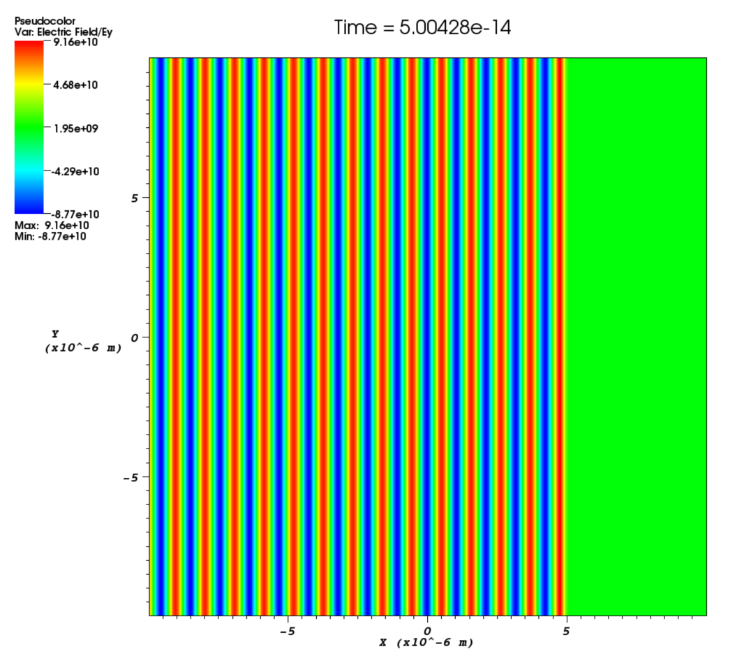
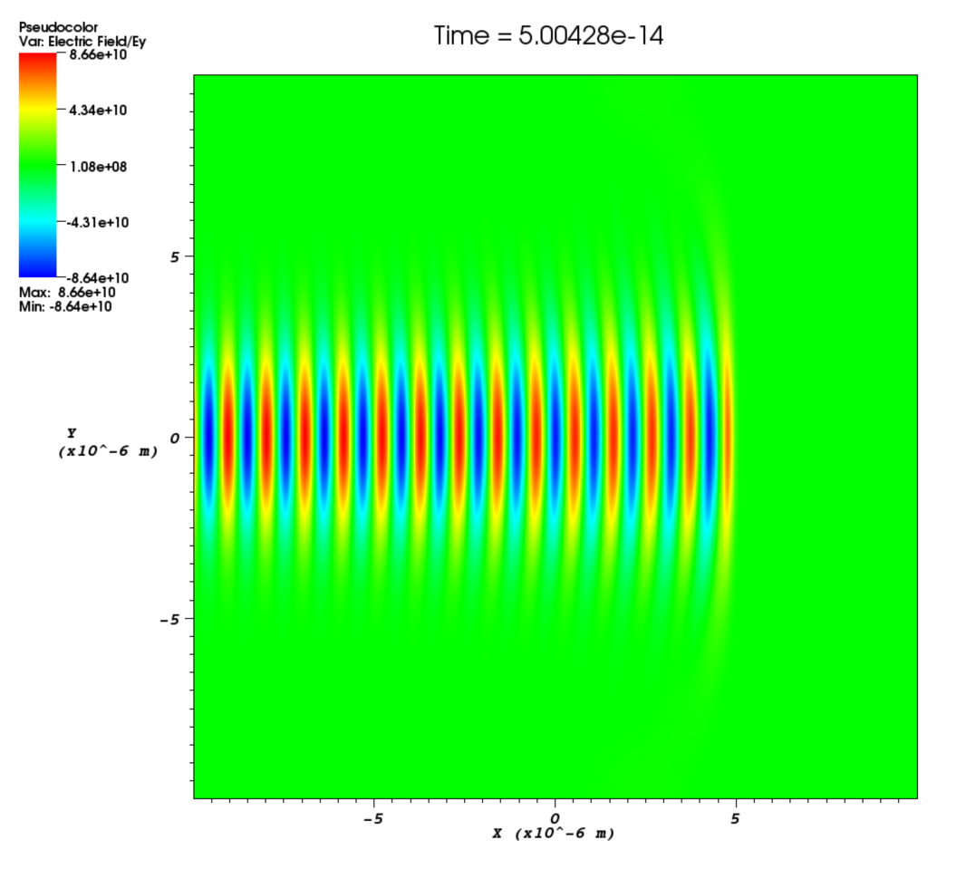
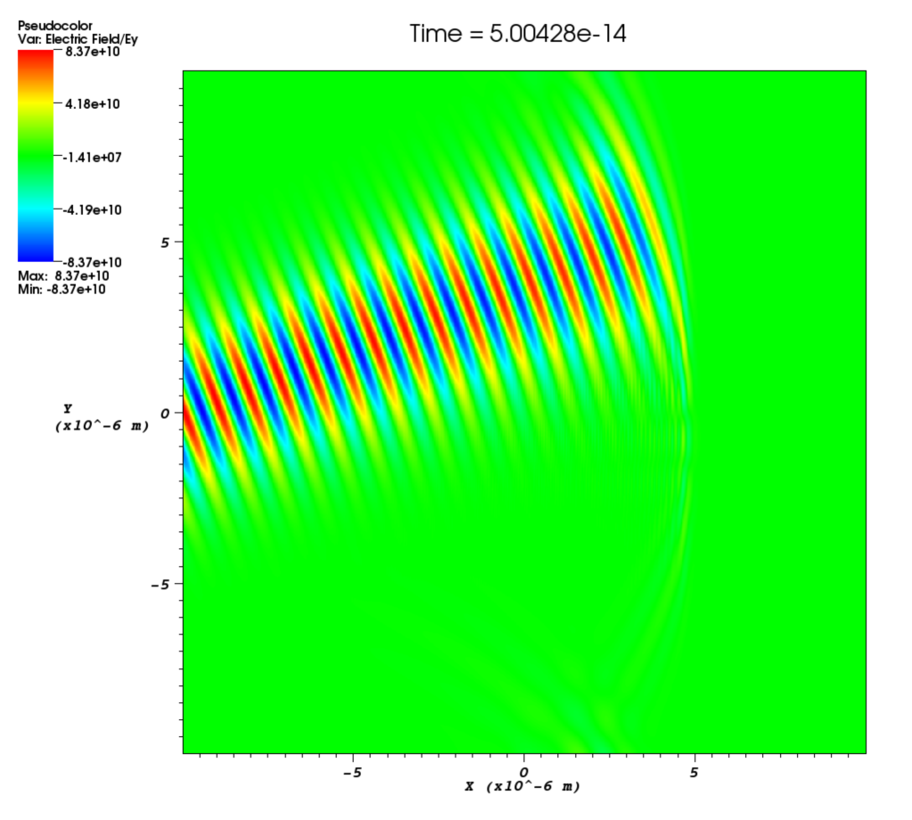
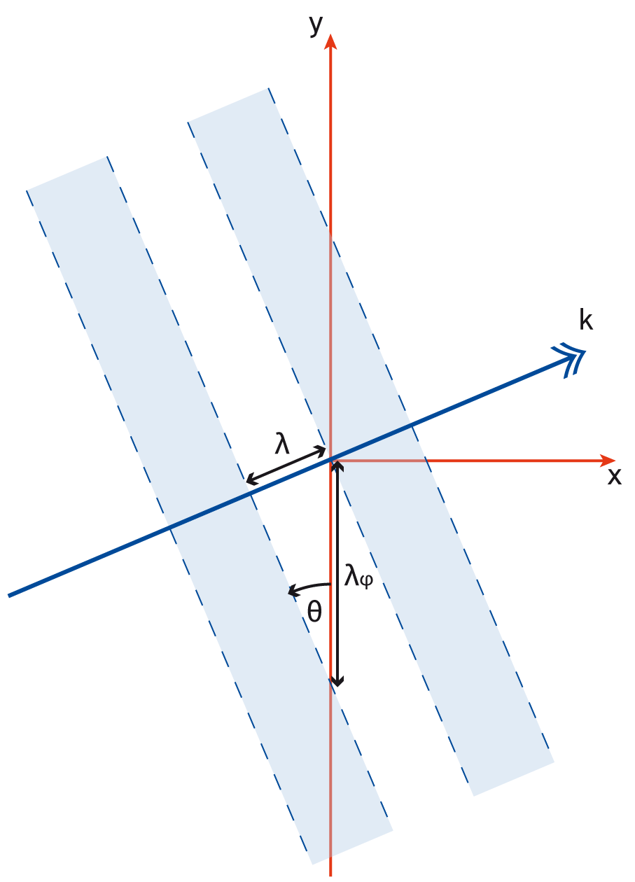
phase- Phase shift for the laser in radians. This is a spatial variable which is also defined across the whole of the boundary on which the laser is attached. This allows a user to add a laser travelling at an angle to a boundary as shown in Figure [angle]. The setup for this is not entirely straightforward and requires a little bit of explanation. Figure [wave] illustrates a laser being driven at an angle on the x_min boundary. Different wave fronts cross the $y$-axis at different places and this forms a sinusoidal profile along $y$ that represents the phase. The wavelength of this profile is given by $\lambda_\phi = \lambda / \sin\theta$, where $\lambda$ is the wavelength of the laser and $\theta$ is the angle of the propagation direction with respect to the $x$-axis. The actual phase to use will be $\phi(y) = -k_\phi y = -2\pi y / \lambda_\phi$. It is negative because the phase of the wave is propagating in the positive $y$ direction. It is also necessary to alter the wavelength of the driver since this is given in the direction perpendicular to the boundary. The new wavelength to use will be $\lambda\cos\theta$. Figure [angle] shows the resulting $E_y$ field for a laser driven at an angle of $\pi / 8$. Note that since the boundary conditions in the code are derived for propagation perpendicular to the boundary, there will be artefacts on the scale of the grid for lasers driven at an angle.
Using this technique it is also possible to focus a laser. This is done by using the same technique as above but making the angle of propagation, $\theta$, a function of $y$ such that the laser is focused to a point along the $x$-axis. A simple example is given here.
Restarting EPOCH from previous output dumps
Another possible way of setting up initial conditions in EPOCH is to
load in a previous output dump and use it to specify initial conditions
for the code. The effect of this is to restart the code from the state
that it was in when the dump was made. To do this, you just set the
field “restart_snapshot” in the
control
block to the number of the output
dump from which you want the code to restart. Because of the way in
which the code is written you cannot guarantee that the code will
successfully restart from any output dump. To restart properly, the
following must have been dumped
- Particle positions.
- Particle momenta.
- Particle species.
- Particle weights.
- Relevant parts of the electric field (If for example it is known that ez == 0 then it is not needed).
- Relevant parts of the magnetic field.
It is possible to use the manual particle control part of the initial conditions to make changes to a restarted initial condition after the restart dump is loaded. The output files don’t include all of the information needed to restart the code fully since some of this information is contained in the input deck. However, a restart dump also contains a full copy of the input deck used and this can be unpacked before running the code. If specific “restart” dumps are specified in the input deck, or the “force_final_to_be_restartable” flag is set then in some cases the output is forced to contain enough information to output all the data. These restart dumps can be very large, and also override the “dumpmask” parameter specified for a species and output the data for that species anyway.
Parameterising input decks
The simplest way to allow someone to use EPOCH as a black box is to give them the input.deck files that control the setup and initial conditions of the code. The input deck is simple enough that a quick read through of the relevant section of the manual should make it fairly easy for a new user to control those features of the code, but the initial conditions can be complex enough to be require significant work on the part of an unfamiliar user to understand. In this case, it can be helpful to use the ability to specify constants in an input deck to parameterise the file. So, to go back to a slight variation on an earlier example:
begin:species
   name = s1

   # First set number_density in the range 0->1
   # Cut down number_density in x direction
   number_density = if ((x gt -1) and (x lt 1), 1.0, 0.2)
   # Cut down number_density in y direction
   number_density = if ((y gt -1) and (y lt 1), number_density(s1), 0.2)

   # Multiply number_density by real particle number density
   number_density = number_density(s1) * 100.0

   # Set the temperature to be zero
   temp_x = 0.0
   temp_y = temp_x(s1)

   # Set the minimum number_density for this species
   number_density_min = 0.3 * 100.0
end:species

begin:species
   name = s2

   # Just copy the number_density for species s1
   number_density = number_density(s1)

   # Just copy the temperature from species s1
   temp_x = temp_x(s1)
   temp_y = temp_y(s1)

   # Set the minimum number_density for this species
   number_density_min = 0.3 * 100.0
end:species
The particle number density (100.0) is hard coded into the deck file in several places. It would be easier if this was given to a new user as:
begin:constant
   particle_number_density = 100.0 # Particle number density
end:constant

begin:species
   name = s1

   # First set number_density in the range 0->1
   # Cut down number_density in x direction
   number_density = if ((x gt -1) and (x lt 1), 1.0, 0.2)
   # Cut down number_density in y direction
   number_density = if ((y gt -1) and (y lt 1), number_density(s1), 0.2)

   # Multiply number_density by real particle number density
   number_density = number_density(s1) * particle_number_density

   # Set the temperature to be zero
   temp_x = 0.0
   temp_y = temp_x(s1)

   # Set the minimum number_density for this species
   number_density_min = 0.3 * particle_number_density
end:species

begin:species
   name = s2

   # Just copy the number density for species s1
   number_density = number_density(s1)

   # Just copy the temperature from species s1
   temp_x = temp_x(s1)
   temp_y = temp_y(s1)

   # Set the minimum number_density for this species
   number_density_min = 0.3 * particle_number_density
end:species
It is also possible to parameterise other elements of initial conditions in a similar fashion. This is generally a good idea, since it makes the initial conditions easier to read an maintain.
Using spatially varying functions to further parameterise initial conditions
Again, this is just a readability change to the normal input.deck file, but it also makes changing and understanding the initial conditions rather simpler. In this case, entire parts of the initial conditions are moved into a spatially varying constant in order to make changing them at a later date easier. For example:
begin:constant
   particle_number_density = 100.0 # Particle number density
   profile_x = if((x gt -1) and (x lt 1), 1.0, 0.2)
   profile_y = if((y gt -1) and (y lt 1), 1.0, 0.2)
end:constant

begin:species
   name = s1

   # Multiply number_density by real particle number density
   number_density = particle_number_density * profile_x * profile_y

   # Set the temperature to be zero
   temp_x = 0.0
   temp_y = temp_x(s1)

   # Set the minimum number_density for this species
   number_density_min = 0.3 * particle_number_density
end:species

begin:species
   name = s2

   # Just copy the number_density for species s1
   number_density = number_density(s1)

   # Just copy the temperature from species s1
   temp_x = temp_x(s1)
   temp_y = temp_y(s1)

   # Set the minimum number_density for this species
   number_density_min = 0.3 * particle_number_density
end:species
This creates the same output as before. It is now trivial to modify the profiles later. For example:
begin:constant
   particle_number_density = 100.0 # Particle number density
   profile_x = gauss(x, 0.0, 1.0)
   profile_y = gauss(y, 0.0, 1.0)
end:constant

begin:species
   name = s1

   # Multiply number_density by real particle number density
   number_density = particle_number_density * profile_x * profile_y

   # Set the temperature to be zero
   temp_x = 0.0
   temp_y = temp_x(s1)

   # Set the minimum number_density for this species
   number_density_min = 0.3 * particle_number_density
end:species

begin:species
   name = s2

   # Just copy the number density for species s1
   number_density = number_density(s1)

   # Just copy the temperature from species s1
   temp_x = temp_x(s1)
   temp_y = temp_y(s1)

   # Set the minimum number_density for this species
   number_density_min = 0.3 * particle_number_density
end:species
This changes the code to run with a Gaussian density profile rather then a step function. Again, this can be extended as far as required.