Weighting Functions

The key feature of a PIC code controlling the smoothness of the solution is the particle shape function. That is the function that describes the assumed distribution of the real particles making up a macro-particle. The simplest solution is to assume that the macro-particles uniformly fill the cell in which the macro-particle is located. This has the advantages of speed and simplicity but produces very noisy solutions. The next simplest approach is to assume a triangular shape function with the peak of the triangle located at the position of the macro-particle and a width of $ 2 \Delta x$, as illustrated below.

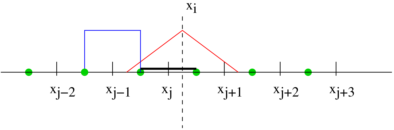
This is the approach used in EPOCH and is a good trade-off between cleanness of solution and speed. Higher order methods based on spline interpolation can be used and do produce smoother solutions, but they are significantly slower and the benefits of the schemes can easily be overstated. EPOCH does now include an option to use 3rd order b-spline interpolation in all parts of the code. This option is enabled with the -DPARTICLE_SHAPE_BSPLINE3 compile time option in the makefile.

Functions derived from the particle shape function appear in two places in the core solver: when the EM fields are interpolated to the position of the macro-particle and when the current is updated and properties of the macro-particle are copied onto the grid. These two uses of the shape function are conceptually similar, but have different forms.

Interpolating grid variables to macro-particles

To derive the equations for calculating the field acting on a particle, you calculate the overlap of the particle shape function with the function representing the fields on the grid. In EPOCH, the fields are approximated at first order so that the field is constant over each cell. Consider a particle with position $X$, where $X$ lies in the cell centred at $x_i$ and grid spacing $\Delta x$. The integral is split into four parts; that part of the shape function which overlaps with the cell $x_{i-1}$, the part of the shape function from the left boundary of $x_i$ to the point of the triangle, the part of the shape function from the point of the triangle to the right hand edge of $x_i$ and finally that part of the shape function which overlaps cell $x_{i+1}$. Assuming that fields are constant inside each cell ($F_i$), this takes the form

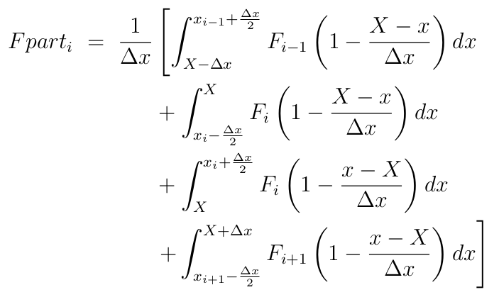
Performing these integrals and remembering that $x_{i-1}+\frac{\Delta x}{2}$ is equal to $x_i-\frac{\Delta x}{2}$ since the grid is uniformly spaced with spacing $\Delta x$, this gives a final formula for the field at a particle of

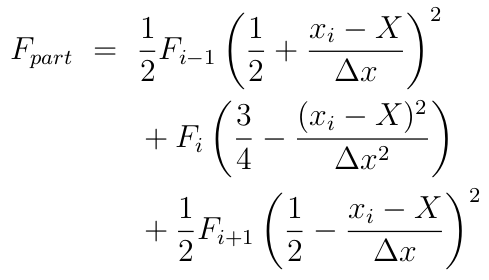
In the code calculating the strength of a cell centred field on the particle is done as follows.

 REAL(num) :: cell_x_r, cell_frac_x
 INTEGER :: cell_x1
 REAL(num) :: gx(-2:2)
 TYPE(particle), POINTER :: current

 part_x  = current%part_pos(1) - x_min_local

 ! Work out the grid cell number for the particle.
 ! Not an integer in general.
 cell_x_r = part_x / dx

 ! Round cell position to nearest cell
 cell_x1 = FLOOR(cell_x_r + 0.5_num)
 ! Calculate fraction of cell between nearest cell boundary and particle
 cell_frac_x = REAL(cell_x1, num) - cell_x_r
 cell_x1 = cell_x1 + 1

 cf2 = cell_frac_x**2
 gx(-1) = 0.25_num + cf2 + cell_frac_x
 gx( 0) = 1.5_num - 2.0_num * cf2
 gx( 1) = 0.25_num + cf2 - cell_frac_x

 f_part = &
       gx(-1) * F(cell_x1-1) &
     + gx( 0) * F(cell_x1  ) &
     + gx( 1) * F(cell_x1+1)

where f_part is the field at the particle location. Note that this has been simplified a little for brevity. Just the triangle shape function is given. In 2D or 3D, you just calculate gy in the same manner as gx and calculate the weight over all the cells affected by the individual 1D shape functions. In 2D this looks like:

 f_part = 0.0_num
 DO iy = sf_min, sf_max
   DO ix = sf_min, sf_max
     f_part = f_part + f(cell_x+ix, cell_y+iy) * gx(ix) * gy(iy)
   ENDDO
 ENDDO

The variables sf_min and sf_max contain the shape function order parameters which indicate the cells each side of the cell containing the particle which are overlapped by the particle shape function. They are defined in shared_data.F90 and should only be changed by the developer if a new particle shape function is being added. Although provided here as pseudo-code for the particle push, it should be noted that the actual particle push unrolls these loops for the sake of speed.

Inside the particle pusher the $E$ and $B$ fields are not cell centred fields, but Yee staggered. This means that there is a small change to the above mentioned example. In 1D this change looks like

 REAL(num) :: cell_x_r, cell_frac_x
 INTEGER :: cell_x1, cell_x2
 REAL(num) :: gx(-2:2), hx(-2:2)
 TYPE(particle), POINTER :: current

 part_x  = current%part_pos(1) - x_min_local

 ! Work out the grid cell number for the particle.
 ! Not an integer in general.
 cell_x_r = part_x / dx

 ! Round cell position to nearest cell
 cell_x1 = FLOOR(cell_x_r + 0.5_num)
 ! Calculate fraction of cell between nearest cell boundary and particle
 cell_frac_x = REAL(cell_x1, num) - cell_x_r
 cell_x1 = cell_x1 + 1

 ! Calculate weights
 INCLUDE 'include/triangle/gx.inc'

 ! Now redo shifted by half a cell due to grid stagger.
 ! Use shifted version for ex in X, ey in Y, ez in Z
 ! And in Y&Z for bx, X&Z for by, X&Y for bz
 cell_x2 = FLOOR(cell_x_r)
 cell_frac_x = REAL(cell_x2, num) - cell_x_r + 0.5_num
 cell_x2 = cell_x2 + 1

 ! Calculate weights
 INCLUDE 'include/triangle/hx_dcell.inc'

 ! bx is cell centred
 bx_part = 0.0_num
 DO ix = sf_min, sf_max
   bx_part = bx_part + bx(cell_x1+ix) * gx(ix)
 ENDDO

 ! ex is staggered 1/2 a cell to the right
 ex_part = 0.0_num
 DO ix = sf_min, sf_max
   ex_part = ex_part + ex(cell_x2+ix) * hx(ix)
 ENDDO

In 2D and 3D, you just combine the shifted and unshifted shape functions and associated cell positions depending on the position of the variable in the cell. Therefore, in 3D and using the loop notation for clarity you would get:

 DO iz = sf_min, sf_max
   DO iy = sf_min, sf_max
     DO ix = sf_min, sf_max
       ex_part = ex_part + hx(ix) * gy(iy) * gz(iz) * &
           ex(cell_x2+ix, cell_y1+iy, cell_z1+iz)
     ENDDO
   ENDDO
 ENDDO

 DO iz = sf_min, sf_max
   DO iy = sf_min, sf_max
     DO ix = sf_min, sf_max
       bx_part = bx_part + gx(ix) * hy(iy) * hz(iz) * &
           bx(cell_x2+ix, cell_y1+iy, cell_z1+iz)
     ENDDO
   ENDDO
 ENDDO

Since $E_x$ is staggered half a grid cell in the x direction, whereas $B_x$ is staggered by half a grid cell in the y and z directions.

Writing macro-particle properties on the grid

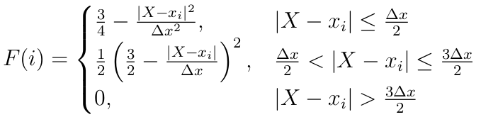
The next stage is to consider how to copy macro-particle properties on the grid. This is very similar to the function for calculating grid variables at the particle location and, for each grid point $x_i$, consists of integrating the part of the particle shape function which overlaps the $i^{th}$ cell. That is

$$ F(i) = Data \int^{x_i+\frac{\Delta x}{2}}_{x_i-\frac{\Delta x}{2}} S(X-x) dx $$

Where $Data$ is the particle property to be copied onto the grid. In EPOCH, since the particle shape function is known to go to zero outside a distance of $2 \Delta x$ from the maximum, the maximum number of cells that can possibly be overlapped by a given particle shape function is 3; the cell containing the particle maximum and the two cells to either side. Performing the integration using the triangular shape function given above gives the result

When this is translated into the code, it looks very similar to that presented for the case where grid properties are interpolated to the particle position. This form is used in the particle pusher to perform the current update and in the routines in src/io/calc_df.F90 to copy particle properties onto the grid for output. The form from calc_df is rather clearer and easier to see in operation. In 1D it looks like:

 cell_x_r = (current%part_pos - x_min_local) / dx + 1.5_num
 cell_x = FLOOR(cell_x_r)
 cell_frac_x = REAL(cell_x, num) - cell_x_r + 0.5_num

 CALL particle_to_grid(cell_frac_x, gx)

 wdata = part_m * fac
 DO ix = sf_min, sf_max
   data_array(cell_x+ix) = data_array(cell_x+ix) + gx(ix) * wdata
 ENDDO

Once again multi-dimensional codes just have the weighting functions multiplied together.

 DO iy = sf_min, sf_max
   DO ix = sf_min, sf_max
     data_array(cell_x+ix, cell_y+iy) = &
         data_array(cell_x+ix, cell_y+iy) + gx(ix) * gy(iy) * wdata
   ENDDO
 ENDDO

Other particle shapes

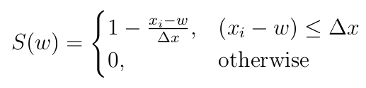
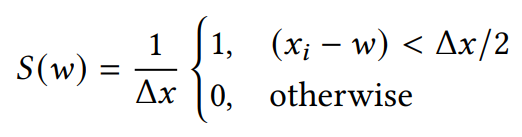
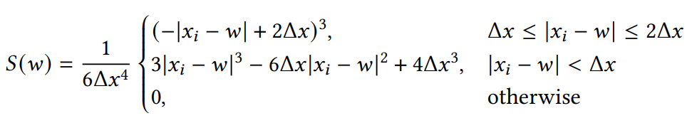
The previous sections dealt with the default macro-particle shape (triangular). EPOCH also supports TOPHAT and BSPLINE particle shapes, although the implementation of these can be different. Interpolating fields to particles and writing particle properties to the grid is performed using the same method as before, but for an altered shape function for TOPHAT:

and for BSPLINE:

In the TRIANGLE and BSPLINE set-ups, the particle shape extends over a size of $2\Delta x$ and $4\Delta x$. Unless the paricle centre is on a cell boundary, the shape will always extend over 3 or 5 cells respectively. However, the TOPHAT shape has a size of $1 \Delta x$, which is an odd number of cell-sizes. If we evaluate this shape at the particle centre, the shape may extend over the cell on the low-$x$ side, or the high-$x$ side. To simplify the code, we evaluate the TOPHAT shape position from the low-$x$, low-$y$, low-$z$ corner of the shape, such that the shape always extends over the current cell and the higher cell only. This is why the cell-calculation for TOPHAT differs from the other shapes, in lines like:

#ifdef PARTICLE_SHAPE_TOPHAT
          cell_x_r = part_x * idx - 0.5_num
          cell_y_r = part_y * idy - 0.5_num
#else
          cell_x_r = part_x * idx
          cell_y_r = part_y * idy
#endif