Parallelism

EPOCH is a massively parallel code written using standard MPI. Due to the massively parallel nature of EPOCH, there are MPI commands scattered throughout many parts of the code, although the MPI has been hidden as far as possible from the end user. The main use of MPI occurs during I/O, in the boundary conditions and during load balancing. The MPI setup routines are all in src/housekeeping/mpi_routines.F90, and the routines which are used to create the MPI types used by MPI-IO are in src/housekeeping/mpi_subtype_control.f90.

General MPI in EPOCH

EPOCH uses Cartesian domain decomposition for parallelism and creates an MPI Cartesian topology using MPI_CART_CREATE. The use of MPI in EPOCH is deliberately kept as simple as possible, but there are some points which must be made and some variables which must be explained.

• MPI decomposition is reversed compared to array ordering. Due to the layout of arrays in Fortran, you get slightly faster performance if you split arrays so that the first index remains as long as possible. Since EPOCH uses MPI_DIMS_CREATE to do array subdivision, this means that the MPI coordinate system is ordered backwards compared to the main arrays. This means that the coordinates array which holds the coordinates of the current processor in the Cartesian topology is ordered as {coord_z, coord_y, coord_x}.
• To make this easier, there are some helper variables. The simplest of these just gives the processors attached to each face of the domain on the current processor. These variables are named x_min, x_max, y_min, y_max, z_min and z_max.
• Since it is possible for particles to cross boundaries diagonally there is another variable neighbour which identifies every possible neighbouring processor including those meeting at single edges and at corners. neighbour is an array which runs (-1:1,-1:1,-1:1) and, perhaps inconsistently, is ordered in normal order rather than reversed order. This means that x_min == neighbour(-1,0,0) and z_max == neighbour(0,0,1).
• The variable comm is the handle for the Cartesian communicator returned from MPI_CART_CREATE.
• The variable errcode is the standard error variable for all MPI communications. However, EPOCH uses the standard MPI_ERRORS_ARE_FATAL error handler so this variable is never tested.
• EPOCH uses a single variable, status, to hold all MPI status calls. Since there is no non-blocking communication this variable is never checked.
• The rank of the current processor is stored in the variable rank.
• The number of processors is stored in nproc.
• The number of processors assigned to any given direction of the Cartesian topology is given by nproc{x,y,z}.

There are some other variables which are not technically part of the MPI implementation, but which only exist because the code is running in parallel. These are

• REAL(num) :: {x,y,z}_min_local - The location of the start of the domain on the local processor in real units.
• REAL(num) :: {x,y,z}_max_local - The location of the end of the domain on the local processor in real units.
• INTEGER, DIMENSION(1:nproc{x,y,z}) :: cell_{x,y,z}_min - The cell number for the start of the local part of the global array in each direction.
• INTEGER, DIMENSION(1:nproc{x,y,z}) :: cell_{x,y,z}_max
• The cell number for the end of the local part of the global array in each direction.

mpi_routines.F90

mpi_routines.F90 is the file which contains all the MPI setup code. It contains the following routines:

• mpi_minimal_init - Contains code to start MPI enough to allow the input deck reader to work. The default EPOCH code setup means that it needs to initialise MPI, obtain the rank and the number of processors.
• setup_communicator - Routine which creates the Cartesian communicator used by the code after the input deck has been parsed. It also populates x_min, x_max etc. It is in its own subroutine so that it can be recalled after the start of the window move when the code is using a moving window. This is needed since it is valid to have a non-periodic boundary before the window starts to move and a periodic boundary afterwards.
• mpi_initialise - This routine calls setup_communicator and then allocates all the arrays to do with fields, etc. It also sets up the particle list objects for each species. If the code is running with only manual initial conditions then this routine loads the requested number of particles on each processor. Otherwise either the restart or the autoloader code load the particles.
• mpi_close - This routine performs all the needed cleanup before the final call to MPI_FINALIZE.

mpi_subtype_control.f90

This file contains all the routines which are used to create the MPI types which are used in the SDF I/O system. Most of the routines in this section are used to create the types used for writing the default variables and, when modifying the code, it is possible to output anything which has the same shape and size on disk as the default variables without ever having to use the routines in this file. However, if you are creating more general modifications which can include variables of different sizes with different layouts across processors then you may wish to use these routines to create new MPI types which match your data layout. Any valid MPI type describing the data layout will work with the SDF library, so there is no absolute need to use these routines. Only the general purpose subroutines are described here, since most of the other routines are fairly clear and use these routines internally.

create_particle_subtype

FUNCTION create_particle_subtype(npart_local)
  
INTEGER(KIND=8), INTENT(IN) :: npart_local

create_particle_subtype is a routine which creates an MPI type representing particles which are spread across different processors with npart_local particles on each processor. npart_local does not have to be the same number on all processors.

Currently this is only used for reading particle data from restart snapshots. It is likely to go away in the near future.

create_ordered_particle_offsets

SUBROUTINE create_ordered_particle_offsets(n_dump_species,&
    npart_local)
  
INTEGER, INTENT(IN) :: n_dump_species
INTEGER(KIND=8), DIMENSION(n_dump_species), &
    INTENT(IN) :: npart_local

create_ordered_particle_offsets is a routine which creates an array of offsets representing particles from n_dump_species which are spread across different processors with npart_local(ispecies) particles of each species on each processor. npart_local does not have to be the same number on all processors and does not have to be the same number for each species.

create_field_subtype

FUNCTION create_field_subtype(n{x,y,z}_local, &
    cell_start_{x,y,z}_local)
  
INTEGER, INTENT(IN) :: nx_local, ny_local, nz_local
INTEGER, INTENT(IN) :: cell_start_x_local
INTEGER, INTENT(IN) :: cell_start_y_local
INTEGER, INTENT(IN) :: cell_start_z_local

create_field_subtype is a routine which creates an MPI type representing a field that is defined across some or all of the processors. The n{x,y,z}_local parameters are the number of points in the x, y, z directions (if they exist in the version of the code that you are working on) that are on the local processor. The cell_start_{x,y,z}_local parameters are the offset of the top, left, back corner of the local subarray in the global array that would exist if the code was running on one processor. This is an offset, not a position and so it begins at {0,0,0} NOT {1,1,1}.

In EPOCH3D there is also a routine called create_field_subtype_2d which is exactly equivalent to create_field_subtype in EPOCH2D and is used for writing the 2D distribution functions. At present, there are not equivalent 1D functions except in EPOCH1D, but these could easily by added if required.

The load balancer

One of the major limiting factors in the scalability of PIC codes is load balancing. Due to the synchronisation of the currents required for the update of the EM fields the entire code runs at the speed of the slowest process. Since most of the time in the main EPOCH cycle is taken by the particle pusher, this equates to the process with the highest number of particles being the slowest. Since the location of particles is dependent upon the solution of the problem under consideration, in general the code will not have exactly the same number of particles on each processor. The load balancer is used to move the inter-processor boundaries so that the number of particles is as close to the same on each processor as possible. The load balancer is invoked at the start of the code and when the ratio of the least loaded processor to the most loaded processor falls below a user specified critical point.

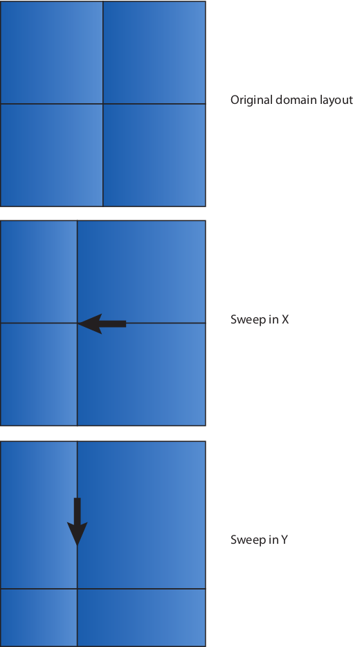
EPOCH’s load balancer works by rearranging the processor boundaries in 1D sweeps in each direction, rather than attempting to perform multidimensional optimisation. Also, at present the MPI in EPOCH requires each processor to be simply connected at every point, so it must have one processor to the left, one to the front etc. which introduces a further restriction on the load balancer. Otherwise, the load balancer is fully general. The load balancing sweep is illustrated here:

The load balancer is implemented in the file src/housekeeping/balance.F90 and is called by the routine balance_workload(override). The parameter override is used to force the code to perform a load balancing sweep even when it would normally determine that the imbalance is not large enough to force a load balancing sweep. Although the load balancer is hard coded to load balance in all available directions, the code is written in such a way that it is possible to modify the code to load balance in only one direction, or to automatically determine which single direction gives the best performance.

The details of the load balancer are fairly intricate, and if major modification to the load balancer is required, it is recommended that the original authors be contacted for detailed advice on how to proceed. However, the general layout of the routine is as follows.

• Use MPI_ALLREDUCE to determine the global minimum and maximum number of particles. If the ratio of the minimum to the maximum is above the load balance threshold then just return from the subroutine.
• The code uses the routines get_load_in_{x,y,z} to determine the work load along each direction of the domain. The get_load_in_x routine uses the x-coordinate of every particle to create a 1D particle density in the x-direction. This is then combined with the total number of grid cells in the y-z plane to give a 1D array of the work load in the x-direction. Similarly for get_load_in_{y,z}.
• Next the load array is passed to the calculate_breaks routine which fills the arrays starts_{x,y,z} and ends_{x,y,z}. These arrays contain the starting and ending cell numbers of the hypothetical global array in each direction for each processor.
• The routine redistribute_fields is then called to move the information about field variables which cannot be recalculated. If new field variables are created that cannot be recalculated after the load balancing is completed then redistribute_fields has to be modified for these new variables.
• The next section of the routine deals with those variables which can be recalculated after the load balance sweep is complete, such as the coordinate axes and the arrays which hold the particle kinetic energy.
• The penultimate section of the routine then changes the variables which tell the code where the edges of its domain lie in real space to reflect the changed shape of the domains.
• The final part is the call to distribute_particles which moves the particles to the new processor. Once this is finished, the code should have as near as possible the same number of particles on each processor.

Most of the load balancer is purely mechanical and should only be changed if the way in which the code is to perform load balancing is fundamentally altered. The redistribution of particles that takes place in distribute_particles uses the standard particle_list objects, so that if the necessary changes have been made to the routines in src/housekeeping/partlist.F90 to allow correct boundary swaps of particles then the load balancer should work with no further modification. The only part of the load balancer which should need changing is redistribute_fields which requires explicit modification if new field variables are required. For fields which are the same shape as the main array there is significant assistance provided within the code to make the re-balancing simpler. There are also routines which can help with re-balancing variables which are the size of only one edge or face of the domain. Variables which are of a completely different size but still need to be rebalanced when coordinate axes move have to have full load balancing routines implemented by the developer. This is beyond the scope of this manual and any developer who needs assistance with development such a modification should contact the original author of the code. The field balancer is fairly simple and mostly calls one of three routines: redistribute_field and either redistribute_field_2d or redistribute_field_1d depending on the dimensionality of your code. To redistribute full field variables the routine to use is redistribute_field, and an example of using the code looks like:

 temp = 0.0_num
 CALL redistribute_field(new_domain, bz, temp)
 DEALLOCATE(bz)
 ALLOCATE(bz(-2:nx_new+3,-2:ny_new+3))
 bz = temp

In this calling sequence the redistribute_field subroutine is used to redistribute the field bz, and the newly redistributed field is copied into temp; an array which is already allocated to the correct size. The new_domain parameter is an array indicating the location of the start and end points of the new domain for the current processor in gridpoints offset from the start of the global array. It is passed into the redistribute_fields subroutine as a parameter from the balance_workload subroutine and should not be changed. The temp variable is needed since Fortran standards before Fortran2000 do not allow the deallocation and reallocation of parameters passed to a subroutine. There is a more elegant solution, where temp is hidden inside the redistribute_field subroutine. However, support for this in current Fortran2000 implementations is unreliable.

The routine for re-balancing variables which lie along an edge of the domain are very similar and are demonstrated in the redistribute_fields subroutine for lasers attached to different boundaries. It is recommended that a developer examine this code when developing new routines.