Field Solver

Each EPOCH MPI rank tracks a separate part of the simulation domain, using arrays of indices (1:nx, 1:ny, 1:nz) in 3D. The MPI ranks also track a small number of cells in neighbouring ranks, such that fields can be interpolated to macro-particle shapes which extend beyond the boundaries of a single rank. These additional surrounding copy-cells are termed “ghost cells”.

Field variables

There are nine variables which are used in updating the EM field solver. These are

• ex - Electric field in the X direction.
• ey - Electric field in the Y direction.
• ez - Electric field in the Z direction.
• bx - Magnetic field in the X direction.
• by - Magnetic field in the Y direction.
• bz - Magnetic field in the Z direction.
• jx - Current in the X direction.
• jy - Current in the Y direction.
• jz - Current in the Z direction.

The EM fields in EPOCH are simple allocatable arrays, which are of size (-2:nx+3,-2:ny+3,-2:nz+3), although this includes the ghost cells. The length of the core domain is different for each variable due to the grid stagger.

The EPOCH field solver is a Yee staggered 2nd order FDTD scheme, directly based on the scheme in the PSC by Hartmut Ruhl and is contained in the file fields.f90. To locate a variable on the grid there is a simple rule.

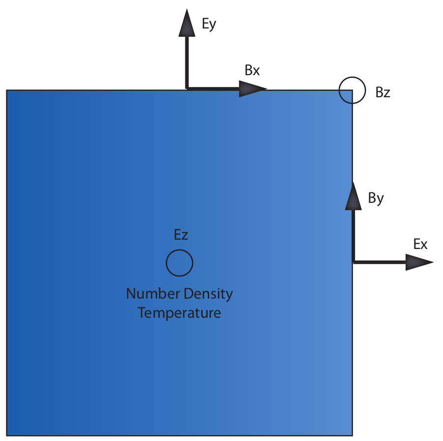
• Start at the cell centre.
• For an $E$ field component, move the field half a grid point in the direction that the field points if possible.
• For a $B$ field component, move the field half a grid point in all directions except the one it points.

This is illustrated below for the 2D case.

The grid stagger means that you have to be careful with boundary conditions since some variables are defined on the domain boundaries whereas others are defined on either side of a domain boundary. This is handled automatically by the built in boundary routines, but must be understood if developing other boundary conditions. To explain it, consider only the left/right boundary in 1D and consider $E_x$ and $B_x$.

$E_x$ is defined on the cell boundary, so ex(0) is the value of $E_x$ on the left boundary and similarly ex(nx) is the value on the right boundary. Conversely, in the 1D code $B_x$ is cell centred (in reality, $B_x$ is never used in the field update and is unimportant since any gradients in $B_x$ in 1D automatically break the solenoidal condition, but this is still a useful example.). This means that bx(1) is the centre of the first cell in the domain, and bx(0) is the value at the centre of the first left hand ghost cell. This means the you must do different things as boundary conditions for the two fields for some boundary conditions.

For example, if you want to clamp the value of $E_x$ to be zero on the boundary, then just set ex(0) = 0.0_num since ex(0) lies on the boundary. To do the same for $B_x$ on the boundary you have to set bx(0) = -bx(1). This is because if you use a linear reconstruction of $B_x$ (i.e second order) then the point between bx(0) and bx(1) has the value $B_x(1/2) = \left(B_x(1)+B_x(0)\right)/2$. Similarly, if you want to set zero gradient on the boundary then for $E_x$ you set ex(-1) = ex(1), whereas for $B_x$ you would set bx(0) = bx(1).

In the particle pusher, time centred field variables are needed for second order accuracy, so an FDTD scheme is used to advance the fields. This looks like

• $\vec{E}^{n+\frac{1}{2}} = \vec{E}^n + \frac{\Delta t}{2} \left( c^2 \nabla \wedge \vec{B}^{n} -\vec{j}^{n} \right)$
• $\vec{B}^{n+\frac{1}{2}} = \vec{B}^n - \frac{\Delta t}{2} \left( \nabla \wedge \vec{E}^{n+\frac{1}{2}} \right)$
• Call particle pusher which calculates $j^{n+1}$ currents
• $\vec{B}^{n+1} = \vec{B}^{n+\frac{1}{2}} - \frac{\Delta t}{2} \left( \nabla \wedge \vec{E}^{n+\frac{1}{2}} \right)$
• $\vec{E}^{n+1} = \vec{E}^{n+\frac{1}{2}} + \frac{\Delta t}{2} \left( c^2 \nabla \wedge \vec{B} ^{n+1} - \vec{j}^{n+1} \right)$

Note that all spatial derivatives are calculated using the staggered grid, so the final derivatives in the code appear one sided. However, this is not the case, and all spatial derivatives are second order accurate. Higher order spatial derivatives schemes for EPOCH are being developed to improve the dispersion properties of the code when resolving small timescales.